Layer-Specific Lipschitz Modulation for Fault-Tolerant Multimodal Representation Learning

1. Introduction: The Hidden Vulnerability of Multimodal Systems

In safety-critical industrial environments, unplanned downtime is more than a technical hurdle—it is a catastrophic economic event. Current estimates attribute massive financial burdens to unscheduled terminations of production, driven by lost production volume, emergency maintenance, and the fracturing of supply chain stability. For decades, the standard defense has been hardware redundancy. The logic was simple: if one sensor fails, another takes its place.

However, this approach possesses a critical blind spot: common-cause failures. Environmental stressors such as extreme heat, mechanical vibration, or high humidity do not target sensors individually; they often degrade or disable multiple redundant components simultaneously, eliminating the safety margin entirely.

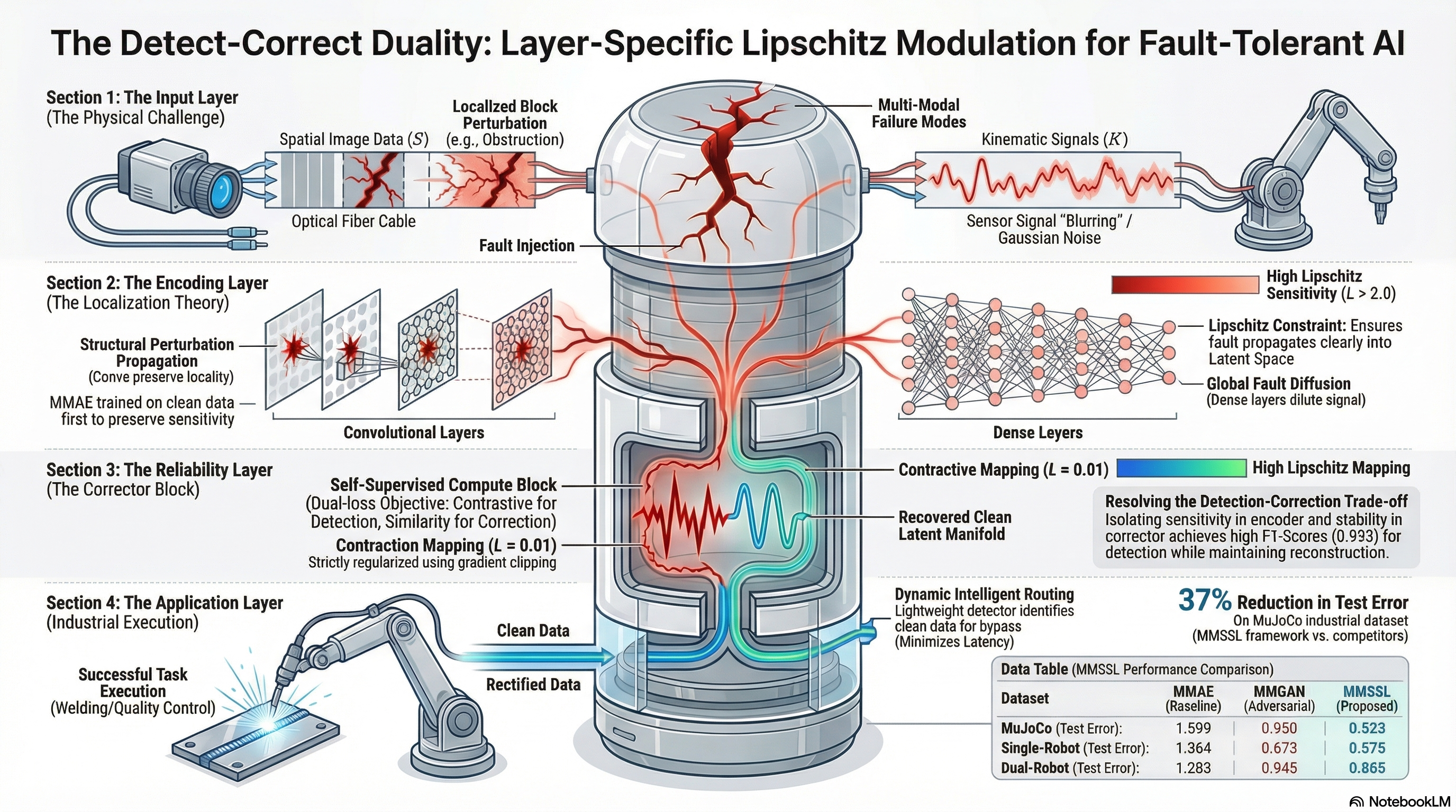
To solve this, we have moved toward multimodal AI systems that fuse heterogeneous data (e.g., camera feeds and kinematic sensors). Yet, these systems face a fundamental “Detection-Correction Trade-off.” Improving a model’s ability to correct errors often requires “smoothing” the latent space, which inherently weakens the signal needed to detect the initial fault. Most architectures optimized for recovery become blind to the anomaly. Our new framework, Layer-Specific Lipschitz Modulation (MMSSL), resolves this by unifying anomaly detection and error correction through the lens of perturbation theory and geometric constraints.

---

2. The Geometry of Failure: Why Architecture Matters

A primary challenge in fault tolerance is understanding how a perturbation—a sensor fault or signal degradation—propagates through a neural network. Theoretical analysis in Lemmas 3.1 and 3.2 reveals that the “Entropy of Fault” is determined by the layer’s structural connectivity.

• Global Diffusion (Dense Layers): Fully connected layers act as global mixing operators. As proven in Lemma 3.1, they distribute fault energy “entropically” across the entire output vector. A localized input perturbation appears as many tiny, diluted signals across the latent space, reducing the per-coordinate salience and making the anomaly “quiet” and difficult for a detector to isolate.
• Spatial Locality (Convolutional Layers): Convolutional layers utilize local receptive fields that preserve geometric coherence. As shown in Figure 10 of our research, these layers are “zero-inflated” (sparse). This locality ensures that perturbation energy remains concentrated in a bounded neighborhood. Because the fault is not diluted, the signal-to-noise ratio remains high, making the anomaly significantly “louder” in the latent space.

---

3. The MMSSL Framework: A Two-Stage Strategy for Robustness

To resolve the trade-off between sensitivity (for detection) and stability (for correction), we employ a two-stage self-supervised training pipeline:

Stage 1: Sensitivity Preservation The multimodal autoencoder is trained exclusively on clean data. By avoiding noise exposure at this stage, we prevent the model from learning to “ignore” perturbations, thereby preserving the encoder’s natural sensitivity to out-of-distribution shifts.

Stage 2: The Compute Block Once the base mappings are fixed, we train a “compute block” to project corrupted latent codes back to a clean manifold using four specialized roles:

1. Encoder: Maps high-dimensional modality inputs to a joint latent space.
2. Detector: Analyzes latent embeddings to output an anomaly score.
3. Corrector: A $L < 1$ contraction mapping that projects distorted features back onto the learned clean manifold.
4. Decoder: Reconstructs the final, rectified signal into the original input space.

---

4. The Mathematical “Secret Sauce”: Lipschitz Modulation & Gradient Scaling

The core innovation is the use of Lipschitz constants ($L$) and Jacobian variation ($L_J$) to control layer-specific sensitivity. While $L_f$ (the first-order term) governs intrinsic sensitivity, Lemma 3.7 shows that input noise modifies the effective Lipschitz constant through curvature-induced sensitivity ($\frac{1}{2}L_J||\delta||^2$).

To optimize the architecture, we apply two opposing forces:

• Selective Gradient Amplification ($\alpha$): In the encoder and detector layers, we scale gradients by $\alpha > 1$. This intentionally increases the local Lipschitz constant, boosting sensitivity to small perturbations to ensure no fault goes unnoticed.
• Gradient Clipping ($\tau$): In the compute block, we enforce a clipping threshold $\tau$ to constrain the Jacobian norm. This ensures the Corrector acts as a stable contraction mapping ($L \approx 0.01$), preventing “gradient explosion” and noise amplification.
• Global Renormalization: To maintain training stability, we implement a global renormalization step after selective amplification. This ensures the total gradient energy remains bounded, preventing the “expansive” detection layers from destabilizing the entire optimization process.

---

5. Empirical Validation: Outperforming the Baselines

We validated MMSSL using the MuJoCo and ABB Robot digital twins. Unlike GAN-based models that rely on stochastic sampling, MMSSL utilizes deterministic geometric projection. This allows for a near-perfect distributional overlap between clean and corrected states in t-SNE manifold analysis, preserving the semantic structure of the data without the risk of “generative hallucinations.”

Table 1: Combined Testing Performance (MuJoCo Dataset, Error in $10^{-2}$)

Model	Camera Error	Sensor Error	Combined Test Error
MMAE	0.145	1.453	1.599
MMFR	0.142	1.318	1.461
MMCF	0.154	0.894	1.048
MMGAN	0.134	0.894	0.950
MMUGAN	0.125	0.779	0.835
MMSSL (Ours)	0.118	0.405	0.523

MMSSL achieved a 37% error reduction over the closest competitor (MMUGAN). In the more complex dual-robot welding datasets, MMSSL outperformed MMCF by 15%, proving its ability to capture intricate kinematic correlations where autoencoders typically suffer from modality collapse. Our low standard deviation ($\pm 0.042$) underscores the reliability of geometric projection over adversarial methods.

---

6. From Theory to Production: The Industrial Pipeline

Deploying MMSSL involves a streamlined three-stage “Operational Pipeline”:

1. Data Ingestion: Heterogeneous streams (Camera, Audio, Kinematic) are encoded into the joint latent space.
2. Intelligent Routing (The Logic Gate): A lightweight detector analyzes the data health. If the signal is “clean,” it bypasses the correction block entirely. This isn’t just for speed; it is about preserving original signal fidelity—preventing unnecessary denoising that could introduce artifacts into healthy data.
3. Downstream Execution: Faulty data is routed through the Lipschitz-regularized Corrector, projecting it back to the clean manifold before passing it to Quality Control or Process Control modules.

---

7. Conclusion: Key Takeaways for AI Safety

Linking perturbation theory to Lipschitz modulation bridges the gap between theoretical guarantees and industrial AI safety. For practitioners, the takeaways are clear:

• Locality is Key: Use convolutional structures in early layers to keep anomaly signals concentrated (sparse) rather than entropic.
• Decouple the Tasks: Separate sensitivity (detection) from stability (correction) through layer-specific Lipschitz and Jacobian constraints.
• Geometry Over Generative Hallucination: Deterministic geometric projection is inherently more stable than GANs for industrial recovery, as it prevents the stochastic “hallucinations” that can lead to physical system failures.
• Scale with Care: Use Selective Gradient Amplification with Global Renormalization to balance the need for high-frequency detection sensitivity with overall training stability.

Read the full paper on arXiv · PDF