Structure-Guided Spatiotemporal Attention Graph Neural Network for Traffic Flow Prediction

1. Introduction: The Risk of Unconstrained Attention in Safety-Critical Systems

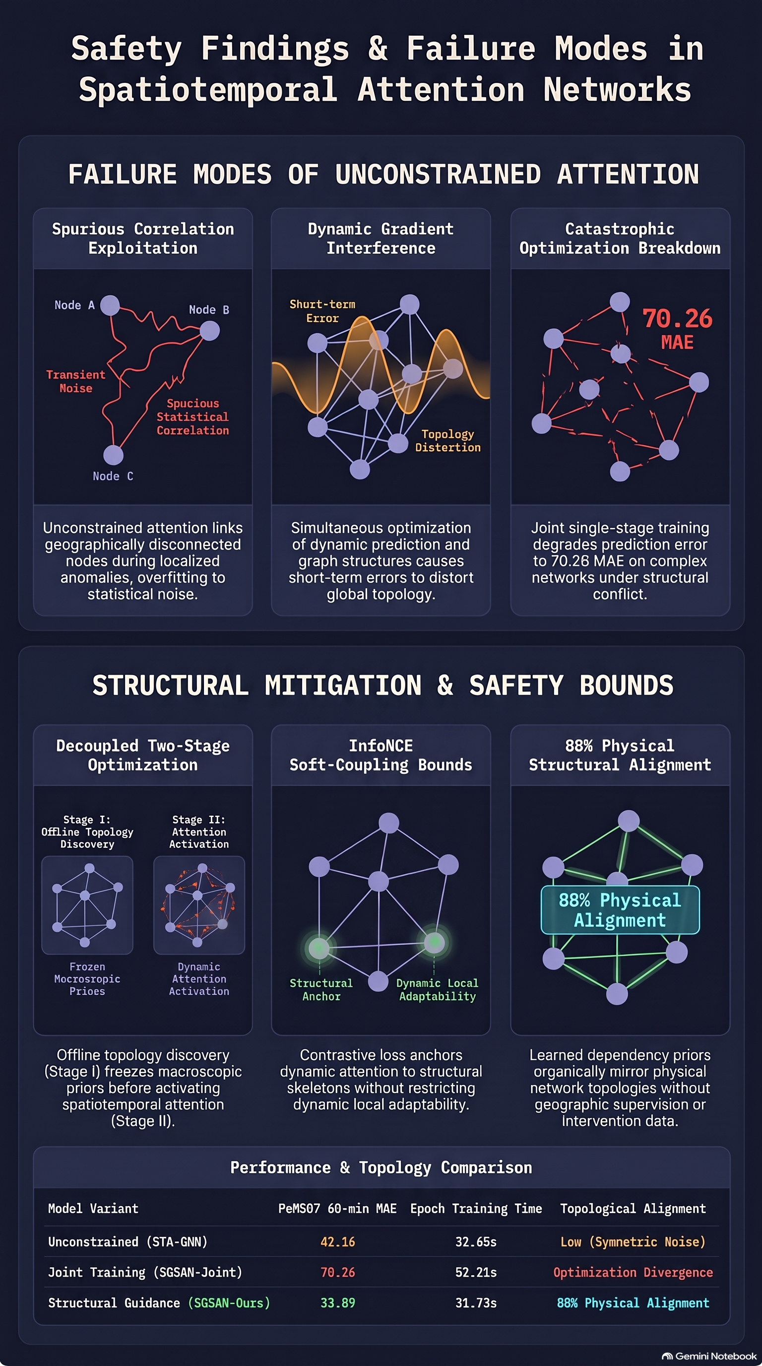
Deep spatiotemporal models integrating graph neural networks and dynamic attention mechanisms have demonstrated remarkable capabilities in modeling complex, non-linear traffic dynamics across network-scale infrastructure. However, deploying these unconstrained, black-box architectures in safety-critical urban systems introduces severe operational risks. Standard dynamic self-attention mechanisms operate in a purely data-driven, correlation-greedy manner: to minimize short-term empirical forecasting errors, they aggregate any available statistical signals across spatial and temporal dimensions.

In complex real-world environments, this unconstrained optimization causes attention mechanisms to latch onto transient observational noise and spurious statistical correlations. For example, a sudden localized rainstorm might create simultaneous, non-physical statistical correlations between two geographically disconnected traffic zones. A standard data-driven attention module will assign high weight to this purely statistical connection despite the total absence of direct physical road infrastructure or traffic propagation between the zones. When environmental conditions change or distribution shifts occur, predictions based on these ephemeral features degrade rapidly, inducing silent operational failure modes that evade standard offline evaluation.

To resolve these vulnerabilities, Xuanmian He, Can Li, and Wanjing Ma introduced the Structure-Guided Spatiotemporal Attention Graph Neural Network (SGSAN). Departing from traditional architectures that rely on unconstrained adaptive graphs or post-hoc diagnostic tools (such as LIME or SHAP)—which merely construct local linear approximations of model behavior without revealing internal reasoning—SGSAN anchors dynamic self-attention to an invariant macroscopic dependency prior. By coupling continuous structural discovery with contrastive mutual information maximization, He et al. establish a framework that preserves real-time predictive precision while providing built-in mechanistic interpretability aligned with the physical logic of physical traffic networks.

---

2. Architecture Breakdown: Anchoring Dynamic Attention to Invariant Structural Priors

The SGSAN framework isolates static topological dependencies from short-term dynamic correlations. The system processes time-series input sequences through a four-module architecture designed to bridge structural discovery with multi-scale spatiotemporal modeling.

Module Name	Underlying Mechanism	Operational Purpose
Temporal Attention Sub-Module	Multi-Head Self-Attention ($Q, K, V$)	Projects historical time-series sequences ($X_{t-T+1:t}$) into temporal node embeddings ($h_t$).
Structural Discovery Module	Continuous DAG-GNN / SEM with NOTEARS trace exponential penalty ($\mathcal{L}_D$)	Learns a static Directed Dependency Graph ($G^*$) capturing time-invariant macroscopic propagation paths ($h_{str}$).
Spatiotemporal Attention Module	Stacked Graph Attention Network (GAT) layers yielding dynamic attention map $G_a$	Captures real-time, dynamic local correlations and short-term temporal fluctuations ($h_{att}$).
InfoNCE Soft-Coupling	Contrastive Mutual Information Maximization ($\mathcal{L}_I$)	Softly anchors dynamic attention to the static topological prior without rigid over-regularization.

Soft-Coupling vs. Rigid Regularization via InfoNCE

A central challenge in spatiotemporal architecture design is maintaining sensitivity to real-time anomalies (e.g., traffic accidents or lane closures) without allowing the dynamic attention mechanism to drift into spurious noise. Traditional constraint mechanisms typically enforce rigid structural bounds via physical distance matrices or strict loss terms like Kullback-Leibler (KL) divergence or Mean Squared Error (MSE). However, these hard constraints force the dynamic attention matrix to rigidly replicate the static graph structure, stripping the model of its representational capacity to adapt to localized, non-topological traffic events.

He et al. address this dilemma by introducing an InfoNCE-based contrastive soft-coupling loss ($\mathcal{L}_I$). The objective function maximizes mutual information between the multi-scale structural representation ($h_{str}$) and the dynamic spatiotemporal representation ($h_{att}$):

$\mathcal{L}_I = -\frac{1}{N} \sum_{i=1}^{N} \log \frac{\exp(\text{sim}(h_{str}^i, h_{att}^i)/\tau_0)}{\sum_{j=1}^{N} \exp(\text{sim}(h_{str}^i, h_{att}^j)/\tau_0)}$

In this formulation, $\text{sim}(\cdot)$ represents the cosine similarity function, $\tau_0$ denotes the contrastive temperature parameter, and $N$ represents the batch size of training samples.

By maximizing cosine similarity between paired representations $(h_{str}^i, h_{att}^i)$ relative to negative sample pairs in a batch, InfoNCE functions as a soft structural alignment guide. It softly anchors the dynamic dynamic attention map ($G_a$) to the stable structural skeleton of the learned Directed Dependency Graph ($G^*$) while preserving the numerical freedom required for the dynamic attention mechanism to capture real-time, localized variances.

---

3. Overcoming Optimization Conflict: The Decoupled Two-Stage Training Framework

Simultaneously training a continuous structural graph discovery module and a deep predictive spatiotemporal attention module introduces severe optimization conflicts. The structural discovery module must filter out short-term noise to isolate a stable, long-term dependency graph. Conversely, the dynamic spatiotemporal attention module greedily minimizes short-term prediction error. When trained end-to-end in a single stage, short-term gradient interference distorts the global dependency graph, resulting in topological instability and severe performance degradation.

To eliminate gradient interference distortion, the authors developed an explicitly decoupled two-stage training strategy:

1. Stage I (DDG Generation): The dynamic spatiotemporal attention module is deactivated. The structural discovery module optimizes continuous directed acyclic graph (DAG) formulations to distill time-invariant macroscopic propagation paths using a joint loss: $\mathcal{L}_{\text{Stage-I}} = \mathcal{L}_A + \gamma_D \mathcal{L}_D + \gamma_S \mathcal{L}_S$

   Where $\mathcal{L}_A$ represents the Mean Squared Error (MSE) prediction loss: $\mathcal{L}_A = \frac{1}{N} \sum_{i=1}^{N} (y_i^t - \hat{y}_i^t)^2$

   $\mathcal{L}_D$ enforces continuous directed acyclicity via the NOTEARS trace exponential penalty: $\mathcal{L}_D = c(V) \cdot [\text{tr}(e^{G \odot G}) - V]$ Here, $\text{tr}(\cdot)$ represents the matrix trace, $\odot$ is the Hadamard product, $e^{(\cdot)}$ is the matrix exponential, and $V$ is the total number of physical detector nodes. A matrix $G$ represents a valid acyclic structure if and only if $\text{tr}(e^{G \odot G}) = V$. To stabilize gradients across varying graph sizes (such as PeMS08 with 170 nodes versus PeMS07 with 883 nodes), the authors introduce a node-dependent scaling coefficient $c(V) = 1 \times 10^{-(V // 10)}$.

   $\mathcal{L}_S$ represents an explicit $L_1$ structural sparsity formulation: $\mathcal{L}_S = \|G\|_1 = \sum_{i=1}^{V} \sum_{j=1}^{V} |G_{ij}|$ This $L_1$ penalty acts as an essential inductive bias, pruning redundant edges to isolate the dominant macroscopic propagation backbone and filter out spurious correlations.

2. Stage II (Soft Alignment): The learned dependency matrix $G^*$ is frozen, serving as a stable structural prior mask. The dynamic spatiotemporal attention module is activated and trained via soft contrastive alignment: $\mathcal{L}_{\text{Stage-II}} = \mathcal{L}_A + \gamma_I \mathcal{L}_I$

Training and Deployment Computational Efficiency

Decoupling graph discovery from dynamic attention optimization achieves marked computational efficiency gains in both offline training and online operational deployment:

• Offline Training Efficiency: Decoupling training dynamics eliminates gradient interference between structural discovery and task loss. Empirical benchmarks demonstrate an average ~31.7% reduction in training time per epoch compared to single-stage joint training. On the large-scale PeMS07 dataset, training latency per epoch decreased from 52.21 seconds (SGSAN (Joint)) to 31.73 seconds (SGSAN (Ours)).
• Online Deployment Efficiency: Continuous DAG optimization carries an $\mathcal{O}(V^3)$ computational complexity, but in SGSAN this process occurs entirely offline during Stage I. During validation and online deployment, the structural discovery module is bypassed. The dynamic spatiotemporal attention module applies the pre-computed sparse topological mask $G^*$. This reduces online spatiotemporal attention complexity from dense computation $\mathcal{O}(T \cdot V^2 \cdot D)$ to $\mathcal{O}(T \cdot |E| \cdot D)$, where $|E| \ll V^2$ represents the sparse edge count.

---

4. Empirical Evaluation: Predictive Accuracy and Operational Latency

He et al. evaluated SGSAN across four standard benchmark datasets from the California Department of Transportation Performance Measurement System (PeMS): PeMS03 (358 nodes), PeMS07 (883 nodes), PeMS08 (170 nodes), and PeMS-Bay (325 nodes).

Comprehensive Forecasting Performance Comparison

SGSAN was evaluated against state-of-the-art spatial-temporal models across 15-minute, 30-minute, and 60-minute forecasting horizons using Mean Absolute Error (MAE), Mean Absolute Percentage Error (MAPE), and Root Mean Squared Error (RMSE).

Dataset	Horizon	Metric	T-GCN	STGCN	GMAN	ASTGCN	STTN	DST2Former	DCST	CCHMM	PSTCGCN	SGSAN (Ours)
PeMS03	15 min	MAE	20.18	17.05	14.87	14.40	16.43	16.53	16.24	23.16	16.40	13.74
		MAPE (%)	19.13	14.41	13.37	12.26	17.38	16.25	13.89	19.85	13.50	11.06
		RMSE	27.82	26.76	23.15	25.17	24.20	25.65	26.17	35.37	24.59	22.56
	30 min	MAE	29.02	26.96	23.65	23.98	22.40	20.41	19.13	33.96	19.46	18.62
		MAPE (%)	26.65	25.99	20.35	20.68	19.12	16.54	17.02	31.04	15.96	15.13
		RMSE	43.36	39.58	36.70	37.71	34.14	32.13	34.19	50.03	29.69	30.71
	60 min	MAE	36.42	31.72	32.00	24.07	27.38	24.72	31.26	28.19	21.53	22.98
		MAPE (%)	33.86	29.73	28.79	20.25	31.77	21.96	28.68	27.87	17.35	18.79
		RMSE	53.03	46.78	47.63	37.65	42.68	37.82	46.41	41.12	33.25	36.74
PeMS07	15 min	MAE	33.66	29.91	26.02	23.29	23.29	24.92	24.34	34.76	26.30	22.84
		MAPE (%)	15.50	12.73	11.47	10.31	11.02	10.94	9.91	15.46	15.99	9.31
		RMSE	47.55	44.41	38.51	35.64	35.47	36.50	36.25	49.87	37.39	35.11
	30 min	MAE	38.72	36.78	34.37	31.42	36.30	29.34	27.99	41.29	31.28	27.47
		MAPE (%)	18.41	16.11	16.64	13.26	16.77	12.37	11.51	20.46	18.46	11.05
		RMSE	54.38	53.62	49.35	46.78	49.95	42.15	41.12	57.58	44.27	40.95
	60 min	MAE	53.37	47.04	47.11	37.41	43.24	38.58	35.78	48.90	40.14	33.89
		MAPE (%)	28.05	23.15	24.90	17.07	19.30	18.82	14.62	22.49	24.50	14.75
		RMSE	73.81	65.69	65.07	53.37	57.50	52.99	51.14	68.31	56.08	50.02
PeMS08	15 min	MAE	21.19	21.35	15.32	15.31	16.41	17.91	16.97	26.80	18.43	14.71
		MAPE (%)	11.76	10.01	9.47	9.13	10.82	9.31	9.78	16.51	13.67	8.59
		RMSE	30.74	30.45	26.55	23.83	23.17	25.89	25.65	39.91	26.70	22.04
	30 min	MAE	28.94	25.75	25.76	22.48	24.11	21.02	21.15	30.69	21.89	19.99
		MAPE (%)	19.17	15.25	16.45	13.08	19.74	12.56	12.77	20.33	15.83	11.74
		RMSE	41.52	37.60	37.16	33.74	33.90	31.50	32.67	44.49	31.72	31.25
	60 min	MAE	44.07	34.06	34.52	29.00	28.11	26.05	25.95	35.67	27.65	20.58
		MAPE (%)	30.77	21.71	22.29	17.19	15.53	16.04	15.75	23.52	19.91	14.60
		RMSE	61.81	47.53	48.46	42.73	40.51	37.19	40.26	49.72	39.66	37.18
PeMS-Bay	15 min	MAE	1.82	1.78	1.63	1.54	1.64	1.54	1.50	1.66	1.93	1.48
		MAPE (%)	3.74	3.49	3.41	3.19	3.39	3.30	3.19	3.43	4.80	3.01
		RMSE	3.40	3.08	3.22	3.18	3.18	2.97	3.01	3.23	4.26	2.70
	30 min	MAE	2.42	2.60	2.20	2.10	2.26	2.17	1.99	2.26	2.45	1.99
		MAPE (%)	5.28	5.66	4.89	4.61	4.64	4.34	4.27	5.05	5.96	4.30
		RMSE	4.71	4.91	4.56	4.42	4.20	3.94	3.99	4.53	5.15	3.87
	60 min	MAE	3.00	3.33	2.95	2.77	2.82	2.61	2.39	3.13	2.95	2.38
		MAPE (%)	6.87	7.53	6.95	6.10	6.17	5.47	5.23	7.31	7.38	5.17
		RMSE	5.74	6.11	6.02	5.81	5.11	5.18	4.76	6.02	6.17	4.60

Ablation Analysis: Structural Variants and Coupling Functions

To systematically isolate the empirical contributions of each architectural component, He et al. conducted extensive ablation experiments across topological configurations and loss coupling formulations.

+-------------------------------------------------------------------------+
|                         Ablation Model Taxonomy                         |
+-------------------------------------------------------------------------+
| Structural Variants:                                                    |
|  - STA-GNN: Structural discovery removed; dynamic attention unconstrained |
|  - DAG-Relaxed: Acyclicity penalty relaxed via tolerance margin epsilon=0.1|
|  - Random-DDG: Learned DDG replaced with random sparse DAG (equal density) |
|  - Joint: Single-stage end-to-end joint training                        |
|                                                                         |
| Coupling Functions:                                                     |
|  - InfoNCE (Ours): Mutual information soft-coupling                     |
|  - KL: Kullback-Leibler divergence hard alignment                       |
|  - Cosine: Direct cosine similarity regularization                      |
|  - MSE: Mean Squared Error structural loss                              |
+-------------------------------------------------------------------------+

1. Structural Prior Removal (STA-GNN): Completely excluding structural discovery degrades predictive performance across all datasets. On PeMS07 at the 60-minute horizon, MAE increases from 33.89 (SGSAN) to 42.16 (STA-GNN), demonstrating that unconstrained self-attention overfits to ephemeral noise.

2. Relaxation of Acyclic Constraints (SGSAN (DAG-Relaxed)): Introducing a tolerance margin ($\epsilon = 0.1$) to the NOTEARS acyclicity loss degrades performance across all horizons (e.g., PeMS07 15-min MAE rises to 28.87). This confirms that strict directed acyclicity is required to prune cyclic statistical noise.

3. Random Graph Injection (SGSAN (Random-DDG)): Substituting the learned DDG ($G^*$) with a random sparse DAG of identical edge density yields worse accuracy than unconstrained attention (STA-GNN) on multiple benchmarks (e.g., PeMS07 15-min MAE of 27.46 vs. 25.52). Performance gains stem from genuine topological discovery rather than simple network sparsity.

4. Single-Stage Joint Training Failure (SGSAN (Joint)): End-to-end optimization without decoupling causes severe gradient interference. On the complex PeMS07 graph, SGSAN (Joint) fails to converge stably, driving the 60-minute MAE up to 70.26.

5. Coupling Function Comparisons (InfoNCE vs. KL, Cosine, MSE): Quantitative results confirm that InfoNCE soft-coupling outperforms alternative structural regularizers across datasets:

   • On PeMS07 (15-min horizon), InfoNCE achieves an MAE of 22.84, compared to KL divergence (28.36), Cosine similarity (24.56), and MSE (28.40).
   • On PeMS03 (15-min horizon), InfoNCE yields an MAE of 13.74, outperforming KL (15.80), Cosine (15.57), and MSE (16.75).

   Rigid constraints like KL divergence and MSE force the dynamic attention matrix to clone the static DDG, destroying representational flexibility. InfoNCE anchors the attention map to the macro skeleton while leaving numerical freedom to capture local real-time variations.

Operational Latency Spectrum

Online inference efficiency tests performed on the PeMS03 dataset demonstrate SGSAN’s computational efficiency relative to representative baseline architectures:

Model	Avg Online Inference Time per Sample (ms)
T-GCN	0.044 ± 0.003
ASTGCN	0.078 ± 0.001
CCHMM	0.079 ± 0.004
SGSAN (Ours)	0.096 ± 0.003
DCST	0.125 ± 0.001
STCGCN	0.136 ± 0.002
DST2Former	0.155 ± 0.002
PSTCGCN	0.434 ± 0.008
SGSAN (Joint)	0.511 ± 0.005
STTN	0.513 ± 0.001

While lightweight baseline architectures like T-GCN (0.044 ms) and ASTGCN (0.078 ms) exhibit lower computational latency, SGSAN (0.096 ms) achieves vastly superior forecasting accuracy while remaining significantly faster than explicit online causal discovery baselines like PSTCGCN (0.434 ms) and un-decoupled joint training models (0.511 ms).

---

5. Mechanistic Interpretability & Physical Network Alignment

To evaluate internal decision-making beyond post-hoc diagnostic approximations, He et al. formulated three quantitative consistency metrics:

1. Attention-Structural Consistency (ASC): Measures internal alignment between the static structural graph ($G^*$) and dynamic attention maps ($G_a$): $\text{ASC} = \frac{1}{B} \sum_{b=1}^{B} \frac{|\text{TopK}(G_a(b)) \cap \text{TopK}(G^*)|}{K}$
2. Structural-Physical Consistency (SPC): Measures external overlap between the learned Directed Dependency Graph ($G^*$) and the true physical road network adjacency matrix ($\mathbf{A}$).
3. Attention-Physical Consistency (APC): Quantifies direct overlap between dynamic spatiotemporal attention maps ($G_a$) and physical road network topology ($\mathbf{A}$).

[ Static Dependency Graph (G*) ] <====== ASC ======> [ Dynamic Attention Map (Ga) ]
                |                                                 |
               SPC                                               APC
                |                                                 |
                v                                                 v
[ ==================== Physical Road Adjacency (A) ==================== ]

Zero-Supervision Physical Alignment

Sensitivity analyses across retained edge thresholds (Top-10% to Top-50% graph capacity) demonstrate that the learned Directed Dependency Graph achieves up to 88% direct structural alignment (SPC = 0.88) with physical road networks (at the Top-30% capacity threshold on PeMS-Bay).

The structural discovery module achieves this physical alignment without receiving any geographic supervision, coordinate metadata, or physical road maps. The architecture distills the physical macroscopic propagation network purely from observational time-series data. Furthermore, APC trajectory curves closely match SPC values across all sparsity thresholds (e.g., at Top-30% on PeMS-Bay, SPC = 0.88 and APC = 0.85), proving that the dynamic attention module inherits physical alignment via InfoNCE coupling.

Subgraph Interpretability & Directional Flow Dynamics

Qualitative subgraph analysis highlights a structural shift in attention distributions between unconstrained models and SGSAN:

Unconstrained Attention (STA-GNN)       Structure-Guided Attention (SGSAN)
     Dense, Bidirectional Edges               Sparse, Unidirectional Paths

           ( Node 184 )                             ( Node 9 )
            ^         |                                  ^
            |         v                                  |
( Node 98 ) <--------> ( Node 5 )                   ( Node 5 ) -------> ( Node 121 )
            ^         |                                  |
            |         v                                  v
           ( Node 21 )                              ( Node 1 )

• Unconstrained Attention (STA-GNN): Subgraph visualizations for key nodes (such as Node 5, Node 21, and Node 44) demonstrate that unconstrained self-attention produces dense, symmetric, bidirectional connections. Node pairs like 5–184 or 21–98 display dense bidirectional arrows, indicating that standard attention merely captures mutual statistical correlations without identifying the physical direction of traffic flow.
• Structure-Guided Attention (SGSAN): Guided dynamic attention inherits the asymmetric, directed properties of the learned DAG prior. Dynamic attention subgraphs reflect unidirectional physical propagation paths: Node 5 cleanly projects influence downstream to Node 9, Node 121, and Node 1; Node 21 propagates to Node 9, Node 1, Node 31, Node 55, and Node 121; and Node 44 propagates downstream to Nodes 1, 9, 26, 55, 80, 101, 121, 144, 219, and 307. Spurious bidirectional statistical edges are eliminated, forcing model decision-making to mirror real-world physical traffic propagation.

---

6. Strategic Takeaways for AI Safety and System Design

The methodology introduced in SGSAN provides actionable architectural principles for research engineers, AI safety red-teamers, and ML practitioners deploying spatiotemporal models in safety-critical domains:

• Anchor Dynamic Learning to Invariant Priors: Unconstrained attention mechanisms greedily optimize for immediate error reduction, making them vulnerable to spurious statistical correlations during distribution shifts. Anchoring dynamic self-attention to learned invariant structural priors prevents representation drift and maintains operational robustness under noisy conditions.
• Decouple Structural Discovery from Task Loss: Combining continuous macro-structural discovery with micro-scale predictive error minimization causes gradient interference distortion. System designers should decouple structural graph discovery into dedicated offline training stages to stabilize global topology learning while reducing online operational inference complexity.
• Prefer Contrastive Soft Coupling over Hard Regularization: Rigid structural constraints (such as KL divergence penalties or hard adjacency bounds) over-regularize neural representations, stripping networks of the flexibility required to adapt to real-time anomalies. Utilizing contrastive mutual information maximization (InfoNCE) provides a soft alignment skeleton while retaining the representational capacity needed for dynamic contextual adaptation.
• Quantify Safety via Mechanistic Consistency Metrics: Evaluating safety-critical networks strictly on post-hoc diagnostics or empirical test set error is insufficient for operational safety. ML systems should be quantitatively audited using internal consistency metrics (such as ASC, SPC, and APC) to verify that internal decision-making processes align with physical domain realities prior to real-world deployment.

Read the full paper on arXiv · PDF