Coverage Aware Active Evaluation for Failure Discovery with Paired Systems

1. Introduction: The Real-World Safety Testing Dilemma

Evaluating safety-critical autonomous systems—such as self-driving vehicles, robotic manipulators, and quadrupedal locomotion platforms—requires discovering rare, severe, and heterogeneous failure modes prior to deployment. However, identifying these edge cases through direct evaluation on high-fidelity target systems (such as physical robot hardware or computationally intensive closed-loop simulators) is severely constrained by strict testing budgets.

To mitigate testing costs, safety evaluation pipelines frequently utilize low-cost proxy systems, including open-loop trajectory playbacks, simplified simulator dynamics, or alternative proxy policies. While proxies enable broad spatial sampling across scenario space, they introduce substantial sim-to-real and system-to-system fidelity gaps. A scenario may trigger a failure in simulation due to simplified contact modeling or visual artifacts while remaining entirely safe on the physical hardware. Conversely, scenarios that appear benign when executed on a proxy evaluator can induce critical, high-severity failures when executed on the target system.

To resolve this trade-off, Parashar et al. (researchers from MIT and NVIDIA Research) proposed a coverage-aware active evaluation methodology in their paper, “Coverage Aware Active Evaluation for Failure Discovery with Paired Systems”. Rather than treating cheap proxies as direct substitutes for ground-truth targets, their framework adaptively uses proxy evaluations to guide target-system sampling. By combining control-variate residual modeling with a support-aware mutual information objective, the methodology maximizes both the discovery rate and spatial diversity of target-system failures under tight target-evaluation constraints.

---

2. The Core Mechanics: Dual-Objective Data Acquisition

The technical architecture proposed by Parashar et al. balances two fundamental goals during scenario acquisition: prioritizing candidate scenarios predicted to trigger high-severity target failures and maintaining spatial exploration across under-covered regions of the scenario space to prevent mode collapse.

                                      [ Candidate Scenarios ]
                                                 │
                                                 ▼
                          ┌──────────────────────────────────────────────┐
                          │         Dual-Objective Acquisition           │
                          │   α(x | D_t) = μ_CV(x) + I(Z_x; R_x | D_t)   │
                          └──────────────────────┬───────────────────────┘
                                                 │
                        ┌────────────────────────┴────────────────────────┐
                        ▼                                                 ▼
     ┌────────────────────────────────────┐             ┌────────────────────────────────────┐
     │ 1. Proxy-Corrected Risk Estimator  │             │ 2. Support-Aware MI Objective      │
     │            (μ_CV(x))               │             │        I(Z_x; R_x | x, D_t)         │
     │ Corrects target surrogate q_θ with │             │ Prioritizes unobserved support and │
     │ correlated proxy signals p(y_s|x). │             │ cluster boundaries to avoid mode   │
     │ Yields minimum-variance estimate.  │             │ collapse.                          │
     └─────────────────┬──────────────────┘             └─────────────────┬──────────────────┘
                       └────────────────────────┬─────────────────────────┘
                                                │
                                                ▼
     ┌────────────────────────────────────────────────────────────────────────────────────────┐
     │                              Batched Acquisition Pipeline                              │
     │ 1. Subsample top-K_MI candidates via Support-Aware MI.                                 │
     │ 2. Filter candidate set Ω_t where μ_CV(x) ≥ γ.                                         │
     │ 3. Select batch b via spatial clustering.                                              │
     │ 4. Evaluate target system, update dataset D_{t+1}, and retrain surrogate model q_θ.    │
     └────────────────────────────────────────────────────────────────────────────────────────┘

2.1 Acquisition Objective Formulation

The decision pipeline evaluates candidate scenarios $x$ drawn from scenario space $\mathcal{X}$ using a dual-objective acquisition function $\alpha(x \mid D_t)$ at iteration $t$, conditioned on evaluated target data $D_t$:

$\alpha(x \mid D_t) = \mu_{CV}(x) + I(Z_x; R_x \mid x, D_t)$

The acquisition function combines a local proxy-corrected risk estimator $\mu_{CV}(x)$ with a support-aware Mutual Information (MI) term $I(Z_x; R_x \mid x, D_t)$ that quantifies scenario diversity and support expansion gain.

2.2 Proxy-Corrected Risk Estimation ($\mu_{CV}$)

Relying exclusively on a target-system surrogate model $q_\theta(x)$ is sample-inefficient because target evaluations are scarce. Parashar et al. incorporate control-variate residual modeling to refine target predictions by combining cheap proxy signals $p(y_s \mid x)$ with learned surrogate predictions.

For a candidate scenario $x$, a local neighborhood $B_x$ is constructed to draw $n$ paired target-surrogate predictions $(\hat{y}_{r,i}, y_{s,i})$ and $k$ additional proxy-only observations $y_{s,j}$. In discrete spaces, $B_x$ represents categorical scenario types, whereas in continuous spaces, $B_x$ is defined as a Euclidean ball $B_x = \{x' \mid \|x - x'\|_2 \le R\}$.

To handle variable predictive variance across the domain, the authors introduce an adaptive neighborhood radius heuristic $R_a(x) \in [R_{\min}, R_{\max}]$. The radius adjusts dynamically based on local sensitivity $s(x)$, which measures surrogate gradient magnitude $\|\nabla_x \mu_q(x)\|$ scaled by predictive variance $\sigma_q(x)$:

$s(x) = \frac{\|\nabla_x \mu_q(x)\|}{\sigma_q(x) + \epsilon}, \quad \tilde{s}(x) = \frac{s(x) - \min_{x'} s(x')}{\max_{x'} s(x') - \min_{x'} s(x') + \epsilon}$

$R_a(x) = R_{\min} + \frac{R_{\max} - R_{\min}}{1 + \exp(\tilde{s}(x))}$

When predictive sensitivity is high, $R_a(x)$ contracts toward $R_{\min}$ to maintain localized accuracy; when sensitivity is low, $R_a(x)$ expands toward $R_{\max}$ to gather broader local context.

Within neighborhood $B_x$, target metric $y_r$ is approximated by target surrogate draw $\hat{y}_r \sim q_\theta(x)$. The proxy-corrected risk estimator $\mu_{CV}(x)$ is formulated as:

$\mu_{CV}(x) = \frac{1}{n} \sum_{i=1}^{n} (\hat{y}_{r,i} - \beta y_{s,i}) + \frac{1}{k} \sum_{j=1}^{k} \beta y_{s,j}$

where adjustment coefficient $\beta$ scales proxy observations based on local covariance:

$\beta = \frac{k}{k+n} \text{Var}(Y_s)^{-1} \text{Cov}(Y_s, Y_r)$

Here, $Y_s$ denotes proxy evaluation metrics and $Y_r$ denotes local surrogate predictions. Parashar et al. prove that conditional on learned surrogate $q_\theta$, this formulation produces an unbiased, minimum-variance local affine estimator of target risk. The local variance of the estimator scales as:

$\text{Var}(\mu_{CV}(x)) = \frac{\text{Var}(Y_r)}{n} \left[ 1 - \frac{k}{k+n} \rho^2(Y_r, Y_s) \right]$

where $\rho(Y_r, Y_s)$ represents the local Pearson correlation coefficient between proxy and target metrics. Whenever proxy evaluations correlate with target behavior ($\rho^2 > 0$), $\mu_{CV}(x)$ strictly reduces estimation variance compared to target-only Monte Carlo sampling.

2.3 Support-Aware Mutual Information (MI) for Diversity

Optimizing solely for risk predictions leads to mode collapse, causing active acquisition to redundantly query minor variations of previously discovered failures. To enforce broad spatial coverage, the framework formalizes scenario diversity using a support-aware Mutual Information (MI) objective.

The evaluated target dataset $D_t$ is partitioned into $K$ spatial clusters. For a candidate scenario $x$, $Z_x \in \{1, \dots, K, \text{new}\}$ represents its cluster assignment variable (where $Z_x = \text{new}$ indicates an evaluation outside existing support), and $R_x \in \{0, 1\}$ represents a binary support discovery variable indicating whether evaluating $x$ reveals novel support. The support-aware MI is formulated as:

$I(Z_x; R_x \mid x, D_t) = H(Z_x \mid D_t, x) - H(Z_x \mid R_x, D_t, x)$

To make this term computationally tractable, the marginal support discovery probability is modeled across clusters:

$p(R_x = 1 \mid x, D_t) = \sum_{k=1}^{K} p(R_x = 1 \mid Z_x = k) p(Z_x = k \mid x, D_t) + p(R_x = 1 \mid Z_x = \text{new}) p(Z_x = \text{new} \mid x, D_t)$

The likelihood $p(R_x = 1 \mid Z_x = k)$ is set to a low likelihood bound $q_k(x) \le \epsilon_{\text{exist}}$ for scenarios within established clusters, whereas for novel support ($Z_x = \text{new}$), likelihood is defined via distance metric $q_{\text{new}}(x)$:

$q_{\text{new}}(x) = \sigma\left(\frac{d_{\text{min}}(x) - \rho}{\gamma}\right), \quad \sigma(z) = \frac{1}{1 + e^{-z}}$

Here, $d_{\text{min}}(x)$ measures distance to the nearest boundary of evaluated support $D_t$. Parameters $\rho$ (novelty radius) and $\gamma$ (softness parameter) are set adaptively from nearest-neighbor distance statistics across evaluated support points $x_i \in D_t$:

$d_{\text{nn}, i} = \min_{j \neq i} \|x_i - x_j\|, \quad \rho = \text{median}(\{d_{\text{nn}, i}\}), \quad \gamma = \text{std}(\{d_{\text{nn}, i}\})$

This geometric parameterization ensures that the MI term assigns maximum information gain to scenarios located far from observed support or lying along ambiguous inter-cluster boundaries.

2.4 Batched Acquisition Pipeline

To make active evaluation computationally efficient under evaluation budget $B = T \cdot b$ (where $T$ is the number of iterations and $b$ is batch size), Parashar et al. structure selection into a four-stage batched acquisition loop (Algorithm 1):

1. Information Subsampling: Evaluate support-aware MI across candidate set $\mathcal{X}$ and select the top-$K_{MI}$ candidate scenarios maximizing $I(Z_x; R_x \mid x, D_t)$. Subsampling via MI acts as a search filter to prune low-information regions prior to computing local control variates.
2. Severity Filtering: Compute local proxy-corrected risk $\mu_{CV}(x)$ for the shortlisted $K_{MI}$ candidates and construct candidate set $\Omega_t = \{x \mid \mu_{CV}(x) \ge \gamma\}$, isolating scenarios estimated to meet or exceed failure threshold $\gamma$.
3. Intra-Batch Spatial Clustering: Partition set $\Omega_t$ into $b$ spatial clusters and select the candidate scenario nearest to each cluster centroid, preventing intra-batch redundancy.
4. Target Rollout & Model Update: Execute target-system rollouts for the selected batch of $b$ scenarios, append results to dataset $D_{t+1}$, and retrain target surrogate model $q_\theta$.

---

3. Empirical Validation Across Autonomous Domains

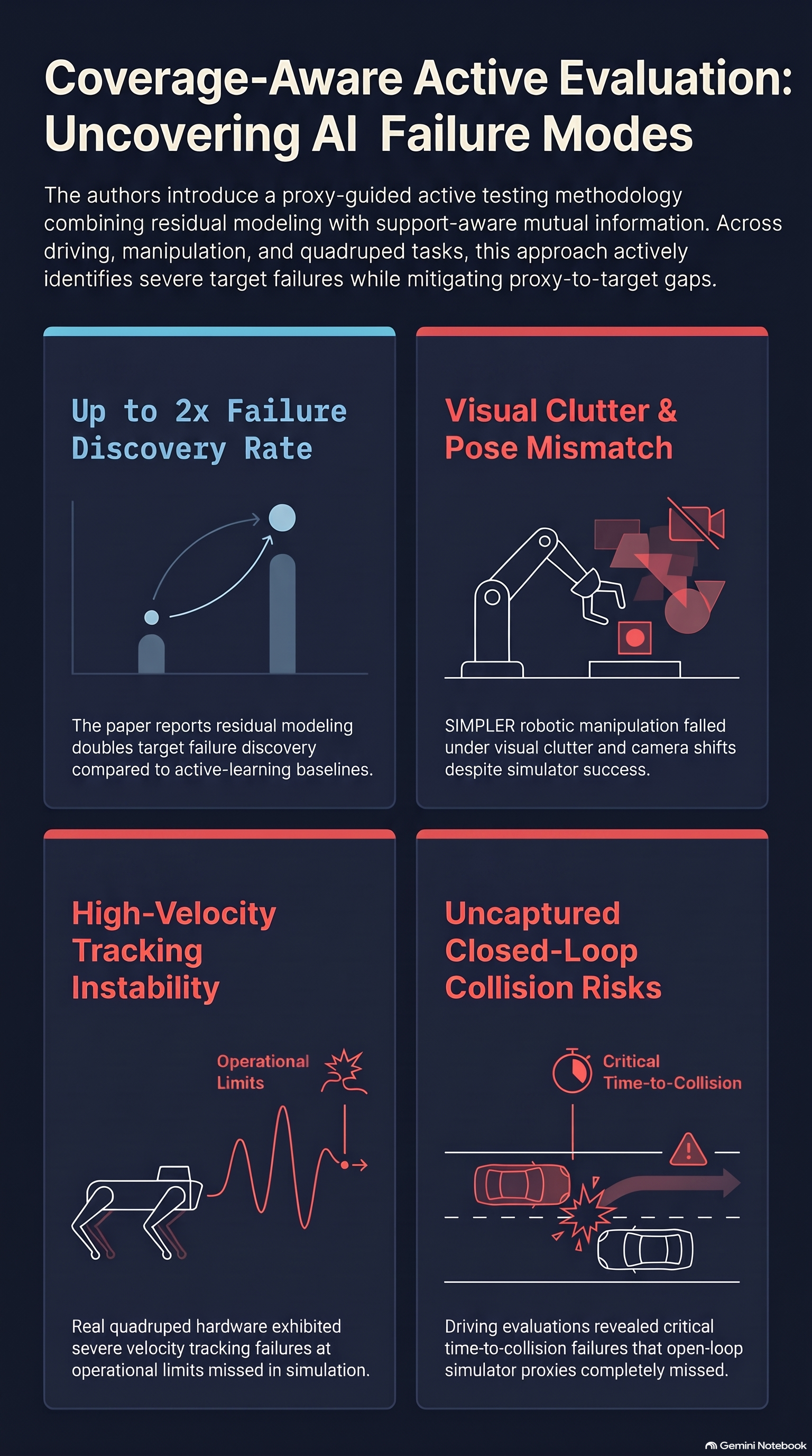
The framework was evaluated across four diverse autonomous system task domains encompassing motion planning, manipulation, legged locomotion, and vision-based perception.

Task Benchmark Summary Table

Benchmark Task	Domain	Scenario Space ($\mathcal{X}$)	Failure Metric ($Y$)	Proxy System	Target System
nuPlan	Autonomous Driving	384-Dimensional feature space	Time-to-Collision (TTC; failure at $\text{TTC} < 0.3\text{s}$)	Open-loop trajectory playback	Closed-loop scenario rollout
SIMPLER	Robotic Manipulation	19-Dimensional space (object pose, distractors, camera)	Grasp success/failure metric ($y=1$ failure)	Photorealistic simulation environment	Environment with visual clutter/occlusion noise
Quadruped	Legged Locomotion	3-Dimensional command velocity ($v_x, v_y, w_z$)	Velocity tracking error (failure at error $\ge 0.7$)	MuJoCo simulation with RL policy	Unitree Go2 quadruped platform / high-fidelity evaluation setup (validated via physical hardware rollouts)
KITTI	Driving Perception	Continuous image scenario space	Ground-truth vehicle coverage continuous score	Virtual KITTI synthetic clone	Real-world KITTI dataset rollouts

Compute Budget Framework

To evaluate methods under equal compute allocations, Parashar et al. define total computational cost as:

$C \approx N_t c_t + N_p c_p$

where $N_t$ and $N_p$ are sample counts, and $c_t$ and $c_p$ represent per-scenario runtimes for target and proxy systems. Proxy sample budgets $N_p$ were adjusted inversely with runtime cost $c_p$. For example, SIMPLER incurs a high proxy runtime ($c_p \approx 83\text{s/eval}$), restricting proxy evaluation to $N_p = 110$ samples. Conversely, Quadruped simulation executes rapidly ($c_p \approx 2\text{s/eval}$), permitting $N_p = 2{,}000$ proxy samples. Target testing budget $N_t = N_0 + B$ remained strictly constrained across all tasks.

Domain-Specific Quantitative Analysis & Results

                  nuPlan Failure Discovery Rate (γ = 0.3)
  ┌─────────────────────────────────────────────────────────────────┐
  │ Proposed   │ █████████████████████████████████████ 0.33          │
  │ BAMS       │ █████████████████████████████ 0.28                 │
  │ BNN-CV     │ ████████████████████████████ 0.27                  │
  │ BNN-C      │ █████████████████████████ 0.25                     │
  │ Random     │ ███████████████████████ 0.23                       │
  └─────────────────────────────────────────────────────────────────┘

• nuPlan Failure Discovery Rates: As detailed in Table 1, the proposed approach discovered significantly more positive failure samples across all severity thresholds $\gamma$ compared to baseline methods under budget $B=170$ ($N_0=20$, $150$ acquired across batch size $b=5$):

  • Table 1: Positive Failure Samples for nuPlan (mean $\pm$ std across four seeds)

    Method	$\gamma = 0.3$	$\gamma = 0.2$	$\gamma = 0.05$
    Random	$0.23 \pm 0.01$	$0.22 \pm 0.00$	$0.21 \pm 0.01$
    BNN-C	$0.25 \pm 0.01$	$0.24 \pm 0.02$	$0.21 \pm 0.02$
    BAMS	$0.28 \pm 0.01$	$0.27 \pm 0.01$	$0.25 \pm 0.01$
    BNN-CV	$0.27 \pm 0.01$	$0.26 \pm 0.01$	$0.22 \pm 0.02$
    Proposed Method	$\mathbf{0.33 \pm 0.01}$	$\mathbf{0.32 \pm 0.01}$	$\mathbf{0.29 \pm 0.01}$

• Quadruped Severity Discovery & Surrogate Accuracy: On the Quadruped task ($B=30$, $N_0=10$, $b=5$), baselines like BAMS clustered near the boundary threshold ($\gamma=0.7$) while missing severe failures. The proposed method discovered severe failures at higher thresholds ($\gamma \ge 1.0$, yield of $0.2 \pm 0.1$, vs. $0.0 \pm 0.0$ for BAMS). Diverse failure discovery directly enhanced surrogate fidelity: the proposed approach achieved $0.80$ mean accuracy over validation failure sets across $\gamma \in \{0.7, 0.8, 0.9, 1.0\}$ (vs. $0.70$ for BAMS) and $0.68$ accuracy specifically on high-severity failure scenarios ($\gamma \ge 1.0$).

• SIMPLER Sim-to-Real Gap & Mode Discovery: SIMPLER exhibited a baseline proxy success rate of 20%, reflecting a substantial sim-to-real gap. The framework successfully isolated two dominant failure modes driven by camera yaw variations ($\theta_{\text{dist}} \in [-\pi, \pi]$ rad) that placed camera positions to the left and right of reference coordinates combined with visual distractor clutter.

• Surrogate Model Agnosticism: The methodology demonstrated adaptability across surrogate neural architectures, utilizing Bayesian Neural Networks (BNNs) for nuPlan, SIMPLER, and KITTI, and Multi-Layer Perceptrons (MLPs) for Quadruped tasks without performance degradation.

Component Ablation Insights

Component isolations conducted on the KITTI vision benchmark (Table 3 in the source paper) reveal the operational necessity of each architectural component:

• Table 2: KITTI Component Ablation Metrics

  Metric	Full Framework	Greedy (No Clustering)	$\beta=0 (n+k)$ Equal-Sample	$\beta=0$ ($n$ Samples)	MI-Only	$-\text{MI-C}$	$-\text{MI-G}$
  Positive Samples ($\gamma=0.5$)	$0.24$	$0.22$	$0.14$	$0.17$	$0.11$	$0.30$	$0.32$
  Positive Samples ($\gamma=0.7$)	$0.03$	$0.01$	$0.02$	$0.01$	$0.02$	$0.02$	$0.01$
  Spatial Coverage Score	$0.78$	$0.58$	$0.79$	$0.72$	$0.91$	$0.60$	$0.48$

• Equal-Sample Proxy Value ($\beta=0(n+k)$): To prove that proxy evaluations provide structural system information rather than merely acting as cheap Monte Carlo samples, the authors evaluated a surrogate baseline receiving $n+k$ target samples without proxy guidance ($\beta=0(n+k)$). At equal sample counts, the full proxy-assisted method achieved a positive sample rate of $0.24$ at $\gamma=0.5$ compared to $0.14$ for $\beta=0(n+k)$. Additionally, proxy guidance expanded meaningful failure mode coverage by nearly 70% and increased surrogate failure recall rate from $0.18$ to $0.49$.

• Support-Aware MI Isolation: Removing MI reduced spatial coverage across all tasks. An MI-only variant achieved high coverage ($0.91$) but low failure discovery ($0.11$ positive samples at $\gamma=0.5$), confirming that spatial exploration without risk estimation wastes evaluation budgets on safe novel states.

• Batch Clustering Isolation: Omitting intra-batch spatial clustering (“Greedy” acquisition) caused coverage on KITTI to drop from $0.78$ to $0.58$ due to intra-batch spatial redundancy and local mode collapse.

---

4. Key Takeaways for AI Red-Teamers & Safety Practitioners

• Proxy Guidance over Proxy Substitution: Low-cost proxies (simulators, open-loop playbacks, related policies) should not be treated as ground-truth evaluators due to persistent sim-to-real gaps. However, discarding proxies entirely discards valuable structural information. Proxy signals are most effective when used adaptively to scale local residual corrections ($\mu_{CV}$) that steer expensive target evaluations.
• Interdependence of Coverage and Risk: Effective safety evaluation requires coupling spatial exploration with target-risk prediction. Pure spatial exploration wastes testing budgets on benign novel states; pure risk optimization without diversity leads to redundant acquisition of identical failure modes.
• Methodology Limitations:
  • Representation Dependency: The framework assumes scenario space representations where spatial locality correlates with system behavior. If feature representations fail to encode behaviorally relevant variations, spatial coverage metrics become less informative.
  • Target Evaluation Scaling: Although proxy guidance significantly reduces target sample requirements, physical or closed-loop target rollouts remain necessary. Complex, high-dimensional scenario spaces still require proportional target evaluation budgets to train accurate target surrogates.

Read the full paper on arXiv · PDF