When Your State Estimator Has Lost The Plot: Detecting Estimator Failures Via Spectral Analysis
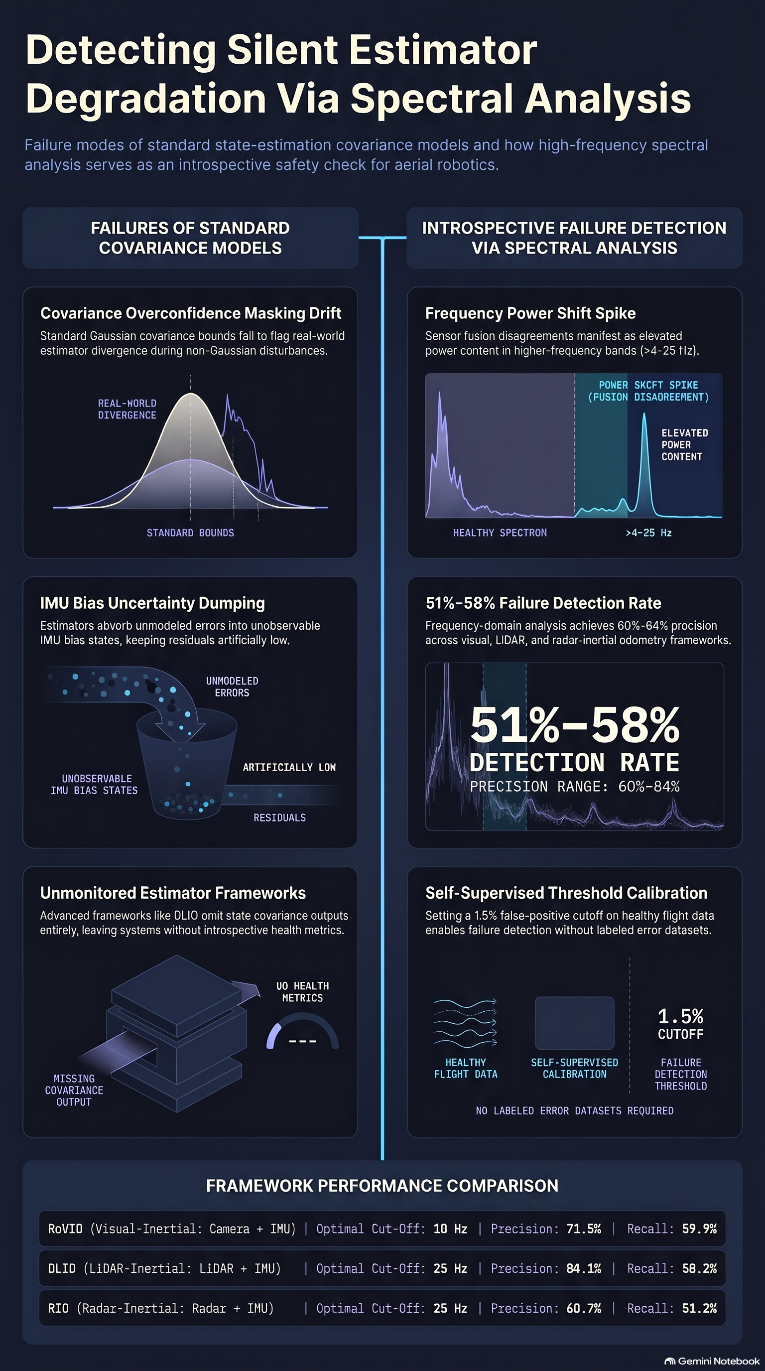
The paper evaluates a sensor-agnostic introspective method that detects state estimator degradation and failure in aerial robotics by analyzing the frequency-domain power distribution of velocity...
1. Introduction: The Blind Spot in Autonomous Perception
Perceptual ambiguity in dynamic environments. Imagine sitting inside a stationary train when an adjacent train begins to accelerate. For a brief instant, visual movement paired with the absence of physical acceleration creates perceptual confusion: is your own train moving, or is the neighboring train departing? Humans resolve this ambiguity almost instantaneously by seeking additional environmental context and evaluating the reliability of their own sensory inputs. This cognitive capability represents a form of real-time perceptual introspection.
The introspective void in robotic systems. Autonomous robotic systems generally lack this level of self-awareness. When operating outside controlled laboratory environments, state estimation algorithms must continuously fuse heterogeneous sensor streams to compute vehicle position and velocity. However, when deployed in unpredictable real-world scenarios, these algorithms are prone to silent degradation or total divergence.
High-stakes operational risks in aerial robotics. The absence of introspective self-monitoring poses critical risks to aerial platforms operating near infrastructure, such as wind turbines or bridges. In close-proximity inspection tasks, minor state estimation errors do not merely cause trajectory drift—they lead directly to physical collisions and catastrophic damage. Furthermore, these platforms encounter rapidly changing operational conditions, including fluctuating illumination, featureless surfaces, spatial constraints, and GNSS outages. Because no single sensor modality functions reliably across all conditions, multi-sensor fusion is mandatory, yet it leaves the state estimator vulnerable to unmodeled disturbances and non-Gaussian sensor defects.
An algorithmic solution for state failure detection. To address this vulnerability, researchers Christian Lanegger, Helen Oleynikova, Roland Siegwart, and Michael Pantic from ETH Zurich and Exclaim Robotics authored the paper When Your State Estimator Has Lost The Plot: Detecting Estimator Failures Via Spectral Analysis.
A sensor-agnostic, lightweight introspective tool. The authors introduce a lightweight, sensor-agnostic introspective framework that evaluates estimator health by analyzing the frequency-domain power distribution of body-frame linear velocity estimates. Operating directly on output dynamics rather than internal state assumptions, the method provides a real-time integrity check for inertially coupled state estimators across visual, LiDAR, and radar modalities.
2. The Limits of Covariance: Why Traditional Health Measures Fail
State estimators traditionally report internal uncertainty using covariance bounds derived from linear filtering or factor graph optimization backends. However, Lanegger et al. demonstrate that these conventional metrics routinely fail to warn operators of impending filter divergence.
The Covariance Trap
Standard state estimation backends model measurement noise using idealized Gaussian assumptions. In real-world field operations, these assumptions are regularly violated by unmodeled disturbances such as sensor aliasing, motion blur, featureless environments, and out-of-distribution noise.
When unmodeled disruptions occur, optimization backends frequently absorb tracking inconsistencies by adjusting unobservable Inertial Measurement Unit (IMU) bias estimates. The backend treats these bias states as a “dumping ground” for uncertainty. Consequently, the optimization algorithm achieves small residuals and outputs low covariance bounds—yielding overconfident bounds—even as true position and velocity drift rapidly multiply.
Lanegger et al. illustrated this phenomenon using an outdoor flight experiment with the visual-inertial odometry (VIO) framework RoVIO. When subjected to aggressive motion blur and featureless surfaces, RoVIO’s true position error diverged severely along its - and -axes at approximately 60 seconds and 120 seconds into flight, despite its reported covariance bounds remaining unrealistically small and confident. Furthermore, many modern state estimation pipelines, such as Direct LiDAR-Inertial Odometry (DLIO), omit state covariance calculations entirely to minimize computational overhead, leaving downstream safety monitors without any internal uncertainty metrics.
Taxonomy of Robust State Estimation Approaches
To contextualize their introspective approach, the authors synthesize existing robust state estimation methods into four distinct operational categories based on how bad measurements are detected and handled:
| Robustness Category | Typical Approaches / Mechanisms | Primary Limitations |
|---|---|---|
| Measurement Rejection | Modality-specific preprocessing; geometric checks on LiDAR point scans; data-driven or self-supervised feature rejection in VIO pipelines. | Tied to specific sensor hardware; fails when unmodeled disturbances bypass front-end validation checks. |
| Measurement Down-Weighting | Backend residual gating via Mahalanobis distance or statistical tests; robust loss functions (M-estimators); Dynamic Covariance Scaling; Gaussian Mixture Models (GMMs). | Assumes Gaussian noise distributions; non-Gaussian alternatives often suffer from backend optimization convergence failures or require hand-tuned parameters. |
| Redundancy & Fallbacks | Running parallel fallback state estimators; local versus global factor graph decomposition; redundant factor graphs for GNSS outages. | Protects against isolated sensor dropouts, but does not measure the health of individual estimators; scales poorly in hardware and computation. |
| Health Monitoring / Introspection | Cross-estimator consensus monitoring; Bayesian nonparametric topic modeling for anomaly detection; Spectral Analysis (Proposed). | Multi-estimator consensus scales poorly with sensor counts; topic modeling struggles to differentiate structural failure from agile flight dynamics. |
3. The Core Mechanism: How Spectral Analysis Detects Estimator Degeneration
The spectral introspection technique formulated by Lanegger et al. relies on physical observations of how inertial sensor fusion backends degrade under pressure.
Physical Intuition and Signal Selection
When an estimation framework combines exteroceptive sensors (cameras, LiDAR, radar) with proprioceptive sensors (IMUs) under degenerate environmental conditions, internal disagreements arise between sensor inputs. This algorithmic tension introduces high-frequency oscillations and “jumpy” noise profiles into the state outputs.
The authors select body-frame linear velocity as the primary signal for spectral monitoring due to three key properties:
- Response Speed: Linear velocity reacts substantially faster to internal estimation stress than accumulated position states.
- Frame Independence: Body-frame velocities do not require global frame alignment, removing transformation estimation errors from the evaluation loop.
- Estimation Dynamics: Unlike angular velocities—which are typically passed directly through from raw IMU gyroscope measurements—linear velocities represent fully integrated fusion outputs.
Signal Processing Pipeline
The continuous introspection framework processes velocity estimates through a five-step signal processing sequence:
- Windowed Sampling: Maintain a sliding temporal window of recent body-frame linear velocity estimates spanning samples over a 1-second duration.
- Segment Detrending: Split the 1-second signal into overlapping segments of length with a overlap (). Subtract the segment mean velocity from each segment to remove DC offsets.
- Windowing Function Application: Apply a Hann windowing function to each detrended segment to minimize spectral leakage and reduce estimator variance.
- Modified Periodogram Computation: Execute Fast Fourier Transforms (FFTs) on each windowed segment to generate individual modified periodograms .
- Welch’s PSD Estimation: Compute Welch’s Power Spectral Density (PSD) estimate by averaging periodograms across all segments over the frequency range .
[ Raw Velocity Time Series (1s) ]
               │
               ▼
   [ Detrending & Windowing ] (Hann Window, 50% Overlap)
               │
               ▼
     [ Fast Fourier Transform ]
               │
               ▼
 [ Welch's PSD Estimation Ŝ_xx[f] ]
               │
               ▼
   [ Band-Limited Metric Extraction ] (Excluding < 10 Hz)
Spectral Metrics
From the estimated PSD, four band-limited frequency-domain metrics are extracted across specified frequency boundaries :
- Total Signal Power (): Integrates total spectral power within the frequency band:
- Spectral Centroid (): Pinpoints the power distribution’s center of mass, identifying the dominant frequency component:
- Spectral Bandwidth (): Quantifies the spread of power content around the spectral centroid:
- Spectral Entropy (): Measures signal irregularity and energy distribution randomness across frequency bins:
Filtering Low-Frequency Nominal Dynamics
Lanegger et al. emphasize that evaluating the full frequency spectrum yields false positives during rapid flight maneuvers. Lower frequencies () are heavily dominated by the robot’s physical motion dynamics; as the platform accelerates, low-frequency signal power increases proportionally even during perfectly healthy state estimation.
By excluding frequencies below a cut-off frequency (), low-frequency motion signatures are filtered out. During nominal operation, healthy estimates contain near-zero high-frequency power. When an estimator degrades, high-frequency spectral power spikes significantly, creating a high-contrast failure indicator.
4. Empirical Evaluation: Performance Across Vision, LiDAR, and Radar
The proposed methodology was evaluated on an outdoor aerial hexacopter platform equipped with a monocular camera, a LiDAR sensor, a radar unit, and an IMU.
Experimental Setup and Labeling
The platform executed 23 minutes of outdoor flight containing real-world edge cases: variable illumination, fast motion, sub-optimal sensor mounting vibrations, onboard computational limits, and dynamic obstacles. Three distinct state estimation frameworks were executed concurrently:
- RoVIO: Iterated Extended Kalman Filter-based Visual-Inertial Odometry (30 Hz).
- DLIO: Direct LiDAR-Inertial Odometry backend (100 Hz).
- RIO: In-house GTSAM factor-graph Radar-Inertial framework (200 Hz).
To establish ground-truth failure labels in the absence of absolute outdoor positioning, the authors applied a consensus-based error windowing technique. Flight data was segmented into 0.1-second intervals. Mean absolute velocity errors were computed across all estimator pairs. An estimator was labeled “healthy” if it agreed with at least one other framework within a velocity error threshold (representing a maximum drift of over 0.1 s). If an estimator deviated beyond relative to both peers, it was labeled “faulty.” Divergent flight segments involving multiple estimators were labeled manually. This process yielded approximately 1.5 minutes of degraded flight data and 17 minutes of healthy flight data (platform velocities spanned , averaging ).
Quantitative Findings
Using precision-recall curve maximization (-score optimization), the authors validated that high-frequency signal power reliably identifies state estimator failure across all evaluated frameworks:
| Estimator Framework | Sensor Modality | Optimal Cut-Off Frequency () | Precision | Recall | PR-AUC |
|---|---|---|---|---|---|
| DLIO | LiDAR-Inertial | ||||
| RoVIO | Visual-Inertial | ||||
| RIO | Radar-Inertial | ||||
| Combined (All) | Multi-Sensor Fusion |
Overall failure detection rates ranged from to across modalities, with precision ranges between and . DLIO achieved the strongest individual detection metrics ( precision at cut-off). Conversely, RIO demonstrated lower precision (), which the authors attribute to higher baseline noise inherent to radar-inertial processing during nominal flight.
Unsupervised Self-Supervised Threshold Strategy
Recognizing that collecting labeled failure data in field deployments is impractical, Lanegger et al. devised a self-supervised thresholding strategy using only healthy flight data:
- Velocity Binning: Healthy flight data is partitioned into velocity bins.
- Relative Power Cut-Off: For each velocity bin, the cut-off frequency is established as the frequency above which power does not exceed of the median total power for that bin.
- Conservative False-Positive Calibration: Detection thresholds are set to bound false positives at a strict false positive (FP) rate on nominal data.
When evaluated across all three estimation frameworks using only healthy data for calibration, the self-supervised strategy achieved performance close to estimator-specific supervised tuning:
- DLIO (1.5% FP): Achieved precision and recall (PR-AUC ).
- RoVIO (1.5% FP): Achieved precision and recall (PR-AUC ).
- RIO (1.5% FP): Achieved precision and recall (PR-AUC ).
Ground-Truth Relative Pose Error Validation
To validate the approach against absolute pose measurements, the authors evaluated high-frequency spectral power against ground-truth Relative Pose Error (RPE) on a dataset running RoVIO. Estimates were partitioned into 0.1-second windows, with failure defined as an RPE exceeding (equivalent to velocity error).
Evaluating signal power above against a threshold of , the spectral analysis method correctly classified estimator health for 85% of the total flight duration. Pronounced power spikes directly aligned with major estimator divergence events at and .
Crucially, this experiment revealed an important edge case: during initial takeoff (), high-frequency power spikes occurred while the platform was stationary or beginning lift-off, despite true geometric position error remaining low. The authors explain that during initial flight phases, IMU biases have not yet converged. Unconverged bias states introduce high-frequency output dynamics into linear velocity estimates, serving as an early indicator of state instability before actual pose divergence manifests.
5. Technical Limitations and Edge Cases
While spectral analysis offers an effective black-box monitoring technique, the authors document several failure modes and physical limitations:
- Smooth Drift and Dropout Invisibility: Spectral introspection depends on high-frequency noise spikes produced by internal filter tension. Smooth, slow-accumulating position drift (such as RoVIO’s gradual divergence) and complete sensor dropouts lack rapid high-frequency power transients. Consequently, under self-supervised parameterization, RoVIO’s recall fell below because slow drift remains spectrally indistinguishable from legitimate low-velocity flight dynamics.
- Takeoff Artifacts and Unconverged IMU Biases: As observed in ground-truth evaluations (), initial takeoff phases where IMU biases have not yet fully converged generate high-frequency power transients. These transients can trigger false positives when geometric position drift remains low, requiring safety monitors to account for initialization settling times.
- Sensor-Specific Baseline Variations: Modality choices impact baseline output dynamics. Radar-Inertial Odometry (RIO) exhibits higher nominal high-frequency spectral power during healthy flight than visual or LiDAR backends. This elevated baseline reduces signal-to-noise contrast between healthy and faulty states, lowering RIO’s failure detection precision.
- Dataset Constraints and Subjectivity: The evaluation dataset reflects real-world operational imbalance, containing far more healthy flight (~17 min) than failed flight (~1.5 min), with a bias toward low-speed hovering ( average). Additionally, consensus labeling introduces boundary ambiguity near the exact onset of state degradation, particularly at low velocities.
6. Key Takeaways & Practical Engineering Implications
- Black-Box Safety Monitoring: Inspecting the high-frequency spectral dynamics of linear velocity outputs provides a lightweight safety monitor. It operates externally, treating the state estimator as a black box without relying on overconfident internal covariances or training data distributions.
- Real-Time Intervention Signals: High-frequency spectral power spikes serve as immediate trigger signals for onboard safety routines. Upon detecting spectral power exceeding calibrated limits, flight control software can initiate corrective actions, such as resetting the filter, switching to secondary fallback factor graphs, deactivating corrupted sensor streams, or triggering safe emergency landing modes.
- Unsupervised Calibration Workflow: Estimator health thresholds can be calibrated without acquiring labeled failure datasets. By analyzing healthy flight data using a relative median power cut-off frequency and a false positive rate threshold, engineers can establish operating limits that perform comparably to supervised methods.
- Accounting for Startup Transients: System designers must account for filter initialization phases. Unconverged IMU biases during startup and takeoff () produce elevated high-frequency spectral power before state convergence, necessitating brief warm-up periods or adaptive thresholding during initial launch.
- Future Development Horizons: Lanegger et al. highlight key avenues for future research, including extending spectral analysis to ground and legged platforms, tracking the spectral characteristics of co-estimated IMU biases directly, and developing dynamic, velocity-dependent thresholding algorithms.
Read the full paper on arXiv · PDF