TravKAN: Fast and Interpretable Nonlinear Traversability Analysis with Kolmogorov-Arnold Networks

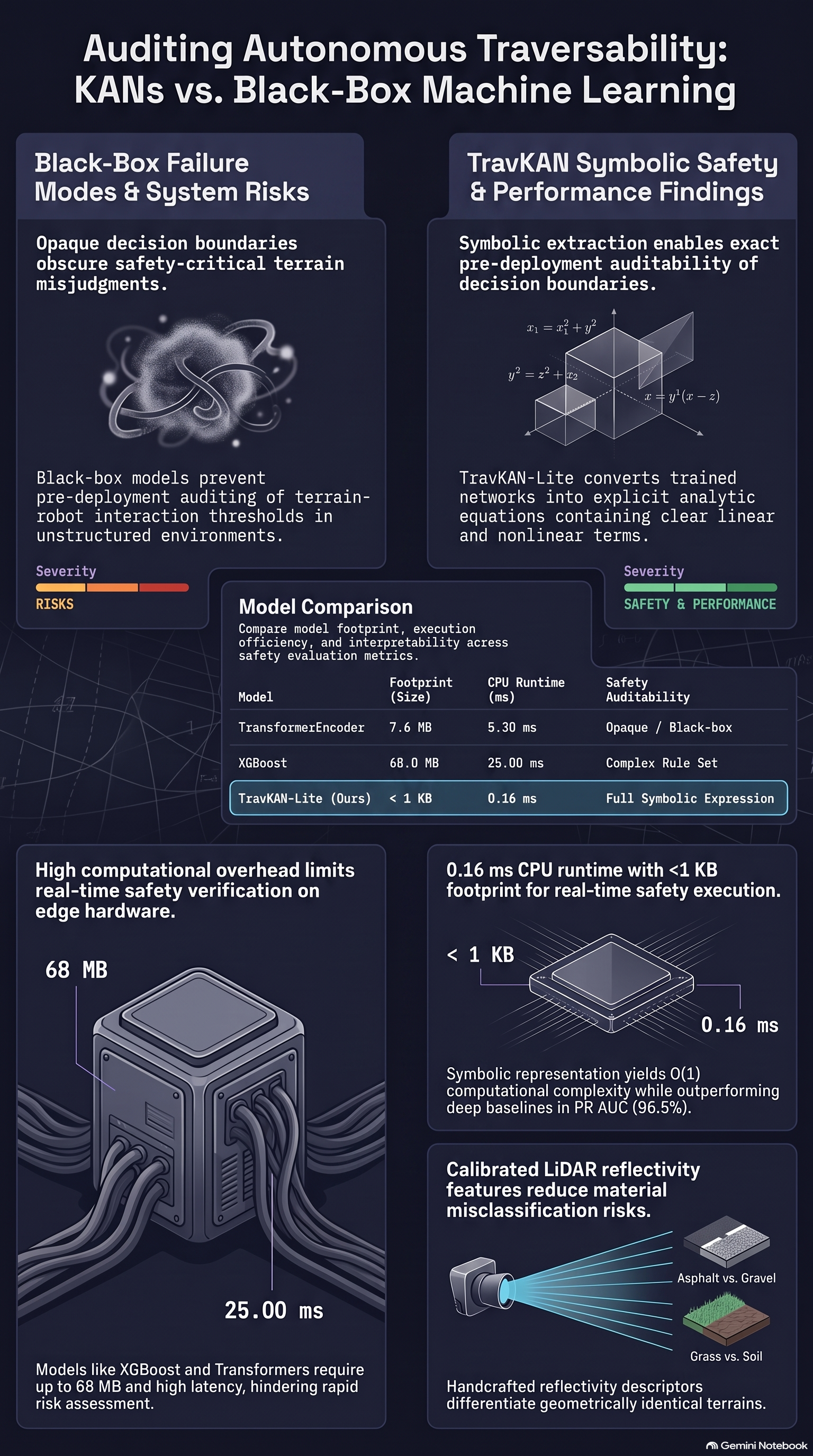
1. Introduction: The Interpretability Deficit in Mobile Robotics

Autonomous mobile vehicles operating in unstructured off-road and semi-structured urban environments must continuously evaluate surrounding terrain to distinguish navigable surfaces from impassable hazards. In a study presented by Fusaro et al., the authors address a critical vulnerability in current data-driven perception pipelines: while modern deep neural networks and tree ensembles achieve strong predictive accuracy, their “black-box” nature obscures why a given terrain patch is classified as traversable or non-traversable. When a deep neural network or gradient-boosted ensemble misinterprets a surface, robotics engineers and safety operators have virtually no visibility into the underlying failure mechanism.

To resolve this interpretability deficit, Fusaro et al. introduce TravKAN, a novel framework based on Kolmogorov-Arnold Networks (KANs) designed for fast, transparent, and scalable terrain evaluation.

Key Concept: Traversability Analysis
Traversability Analysis is the process of estimating a terrain patch’s traversability score—determining whether an autonomous ground vehicle can safely traverse a given region without getting stuck, tipping over, or suffering physical damage.

The primary contributions established by Fusaro et al. include:

• Kolmogorov-Arnold Networks for Traversability: The first application of KANs to terrain evaluation, replacing static node activation functions with learnable univariate edge functions.
• LiDAR Reflectivity Descriptors: A novel set of handcrafted features derived from the LiDAR reflectivity channel, capturing intrinsic surface reflectance properties that complement standard geometric and remission cues.
• Symbolic Model Extraction (TravKAN-Lite): A procedure for converting learned B-spline edge transformations into explicit, closed-form analytic expressions, yielding an auditable, deployment-friendly representation with $O(1)$ runtime complexity.

---

2. Deep Dive: Architectural Mechanics of TravKAN

Standard Multilayer Perceptrons (MLPs) parameterize multivariate functions by applying linear weight matrices followed by fixed activation functions ($\sigma$, such as ReLU or GELU) placed at network nodes:

$f(x) = W_L \sigma(W_{L-1} \sigma(\dots \sigma(W_1 x)))$

In standard MLPs, expressivity is concentrated within the weight matrices, while nonlinearities remain globally shared and static.

In contrast, Kolmogorov-Arnold Networks invert this parameter structure by placing learnable univariate functions ($\phi_{ij}$) directly on network edges. Motivated by the Kolmogorov-Arnold superposition theorem, a KAN layer mapping $\mathbb{R}^n \to \mathbb{R}^m$ computes:

$z_j = \sum_{i=1}^{n} \phi_{ij}(a_{ij} x_i + b_{ij}), \quad j = 1, \dots, m$

where $a_{ij}, b_{ij} \in \mathbb{R}$ are learnable affine scalars, and $\phi_{ij} : \mathbb{R} \to \mathbb{R}$ are learnable univariate functions.

To parameterize each $\phi_{ij}$, TravKAN employs B-spline basis expansions over local intervals $[-1, 1]$ with grid resolution $G$:

$\phi_{ij}(t) = \sum_{k=1}^{G} c_{ijk} B_k(t)$

Because B-splines possess local support and $C^{r-1}$ smoothness, local parameter adjustments do not trigger global representation collapse across the full input domain. For failure-first autonomous systems safety, this local support property provides a vital safeguard against catastrophic interference: modifying the model to correct a localized failure mode on a specific terrain type (such as mud patches or tall grass) will not corrupt learned decision boundaries for distinct, previously validated terrain types (such as asphalt or flat gravel).

To scale model capacity without widening layer dimensions, Fusaro et al. implement a 3-step grid refinement training protocol:

1. Step 1: Initial training with grid resolution $G = 8$ for 50 epochs using AdamW (initial learning rate 0.005).
2. Step 2: Grid refinement to $G = 40$ for 30 epochs with a linearly decreased learning rate (decay coefficient 0.125).
3. Step 3: Final grid refinement to $G = 48$ for 20 epochs with further linear learning rate decay (coefficient 0.125).

TravKAN utilizes a lightweight architecture defined by hidden dimension constraints $[n_{in}, n_{hidden}, n_{out}] = [d, 24, 2]$, where $d$ is the feature dimensionality. This shallow configuration restricts the total parameter count to approximately 10,000 (10K), maintaining a lightweight 72 KB memory footprint.

Architectural Feature	Traditional MLPs	Kolmogorov-Arnold Networks (TravKAN)
Nonlinearity Location	Fixed on nodes ($\sigma$)	Learnable functions on edges ($\phi_{ij}$)
Activation Parameterization	Static functions (e.g., ReLU, GELU)	B-spline basis expansions ($B_k$)
Capacity Scaling	Layer width and depth expansion	Local grid resolution ($G$) refinement
Interpretability	Opaque “Black-Box” matrix operations	Explicit symbolic decomposition into analytic functions

---

3. Beyond Geometry: Unlocking LiDAR Reflectivity Features

To complement geometric and remission descriptors, Fusaro et al. introduce a feature set derived from the LiDAR reflectivity channel. The authors detail a fundamental physical distinction between remission and reflectivity:

• Remission: Raw returned signal intensity influenced heavily by target distance, sensor-specific characteristics, and beam incidence angles.
• Reflectivity (Calibrated Intensity): An intrinsic surface reflectance measurement calibrated to eliminate range and angular attenuation dependencies.

While terrain types such as asphalt and gravel or wet grass and dark soil often exhibit identical geometric profiles or overlapping raw remission values, their physical surface reflectances differ.

To capture these material cues, the authors project the point cloud $P$ onto the ground plane and discretize it using a polar grid $G = \{C_k\}_{k=1}^M$. Within each polar cell $C_k$, handcrafted features are aggregated into a cell-wise descriptor vector:

• Feature Vector Composition: $v_k = [v_k^{geom}, v_k^{remission}, v_k^{reflectivity}]$
  • Geometric Descriptors ($v_k^{geom}$): Spatial statistics capturing elevation, local surface normal ($nv_z$), slope angle, roughness, unevenness, surface density, and point distribution.
  • Remission Descriptors ($v_k^{remission}$): Minimum, maximum, mean, and variance of raw intensity returns.
  • Reflectivity Descriptors ($v_k^{reflectivity}$): Minimum, maximum, mean, variance, dispersion of calibrated reflectivity within the cell, and radial distributional measures.

The input feature dimension $d$ varies across benchmark datasets based on feature availability:

• EastPark Dataset ($d = 36$): Incorporates geometric, remission, and the newly calculated reflectivity descriptors (which were specifically collected and engineered for the EastPark benchmark).
• SemanticKITTI & nuScenes Datasets ($d = 29$): Incorporates geometric and remission descriptors, as public standard benchmarks only provide standard remission channels.

---

4. TravKAN-Lite: Symbolic Extraction and Auditability for AI Safety

For safety-critical autonomous systems, verifying model safety requires inspecting decision boundaries prior to physical deployment. Because KANs parameterize univariate edge transformations via explicit B-splines, trained networks can be converted directly into closed-form mathematical equations, producing a symbolic model termed TravKAN-Lite.

After training, B-spline curves are converted into explicit analytic functions (comprising linear, quadratic, exponential, trigonometric, rational, and composite terms). On the EastPark dataset, symbolic extraction yields a decision function structured as:

$\hat{y} = L(x) + Q(x) + E(x) + S(x) + R(x) + C(x) + b$

where $x \in \mathbb{R}^d$ is the feature vector, $b$ is the scalar bias, and $L(x), Q(x), E(x), S(x), R(x), C(x)$ represent linear, quadratic, exponential, trigonometric (sine/cosine), rational, and composite interaction terms, respectively.

An algebraic analysis of the extracted symbolic expressions reveals the structural logic of the decision boundary:

1. Dominant Base Predictors: Local height statistics ($z_{ave}, z_{var}, z_{std}, z_{min}, z_{max}$) and average intensity possess the largest linear and base coefficients, driving the core terrain classification.
2. Nonlinear Local Corrections: Secondary geometric descriptors, such as surface normal vertical component ($nv_z$), slope angle, unevenness, and surface density, appear primarily within nonlinear, composite, and trigonometric basis functions. These act as conditional local correction terms under specific terrain configurations rather than applying uniform global weights.

This symbolic transparency allows safety auditors to inspect nonlinear decision boundaries, evaluate terrain-robot interaction thresholds offline, and perform deterministic edge-case verification without relying on empirical black-box testing.

---

5. Empirical Evaluation: Performance, Latency, and Memory Footprint

Fusaro et al. evaluated TravKAN and TravKAN-Lite across three public LiDAR benchmarks: EastPark (off-road and urban), SemanticKITTI (dense urban driving), and nuScenes (multi-city driving). Baseline comparisons include Multi-Layer Perceptrons (MLP, MLP++), a 6-layer TransformerEncoder, a Pyramidal 3D SVM (P-SVM), and XGBoost (3,000 trees).

Evaluated on an Intel Core i7-7700K CPU and NVIDIA Titan RTX GPU (considering an average of ~1,100 polar cells per frame on EastPark, excluding the ~6 ms shared feature extraction time), Table 1 details computational overhead and execution latencies across models.

Table 1: Model Efficiency and Deployment Benchmarks

Method	Parameters	Model Size	CPU Time (ms/frame)	GPU Time (ms/frame)
MLP	61K	244 KB	0.9 ms	0.4 ms
MLP++	62K	260 KB	1.4 ms	0.7 ms
TransformerEncoder	2M	7.6 MB	5.3 ms	4.3 ms
P-SVM	30K	25 MB	50 ms	N/A
XGBoost	560K	68 MB	25 ms	N/A
TravKAN	10K	72 KB	71 ms	60 ms
TravKAN-Lite	<1K	<1KB	0.16 ms	N/A

While standard TravKAN exhibits higher CPU/GPU inference latency due to B-spline evaluation overhead, its extracted symbolic counterpart, TravKAN-Lite, reduces parameter count to under 1,000, shrinks memory to under 1 KB, and executes in 0.16 ms per frame on CPU—representing a speedup of over two orders of magnitude with deterministic $O(1)$ computational complexity.

Table 2: Comprehensive Cross-Dataset Performance Comparison

Dataset	Method	Balanced Accuracy (%)	mIoU (%)	F1 Score (%)	ROC AUC (%)	PR AUC (%)
EastPark	MLP	87.6	80.3	88.8	89.8	94.1
	MLP++	87.9	77.8	87.2	92.2	95.6
	TransformerEncoder	87.9	79.4	88.2	91.9	95.4
	P-SVM	87.6	82.0	90.0	90.7	94.7
	XGBoost	87.4	79.5	88.3	88.6	92.2
	TravKAN	87.8	77.6	87.0	93.1	96.5
	TravKAN-Lite	85.6	77.5	86.9	89.0	93.9
SemanticKITTI	MLP	84.0	67.6	80.6	92.1	83.2
	MLP++	93.9	87.9	93.5	98.1	96.6
	TransformerEncoder	89.7	78.8	88.1	95.8	92.5
	P-SVM	91.2	87.1	93.1	96.3	97.0
	XGBoost	93.4	87.3	93.2	98.3	96.9
	TravKAN	93.5	86.2	92.5	98.4	97.1
	TravKAN-Lite	86.3	71.2	83.1	89.0	69.8
nuScenes	MLP	93.1	87.0	93.1	97.4	95.6
	MLP++	95.8	91.9	95.8	99.0	98.7
	TransformerEncoder	83.1	66.4	79.7	90.8	82.1
	P-SVM	93.4	89.9	93.2	97.9	96.9
	XGBoost	95.6	91.6	95.6	99.1	98.9
	TravKAN	95.7	91.7	95.7	99.1	98.9
	TravKAN-Lite	89.4	80.2	89.1	95.0	91.3

Textual and Ablation Analysis

• Ranking Robustness & Cross-Domain Generalization: On EastPark, TravKAN achieves top-tier ranking metrics with 96.5% PR AUC and 93.1% ROC AUC, outperforming XGBoost (92.2% PR AUC, 88.6% ROC AUC) and deep baselines. On nuScenes, a notable contrast emerges: while the over-parameterized TransformerEncoder severely degrades to 83.1% Balanced Accuracy and 90.8% ROC AUC, TravKAN maintains strong cross-city generalization at 95.7% Balanced Accuracy and 99.1% ROC AUC (matching XGBoost).

• Reflectivity Feature Ablation: On EastPark, evaluating feature subsets reveals a subtle physical interaction:

  • Geometry Only (geom): 87.4% Bal. Acc, 92.7% ROC AUC, 96.4% PR AUC.
  • Geometry + Remission (geom+remission): 87.5% Bal. Acc, 92.6% ROC AUC, 96.3% PR AUC.
  • Full Model (Full TravKAN): 87.8% Bal. Acc, 93.1% ROC AUC, 96.5% PR AUC.

  Adding raw remission to geometry slightly decreases ROC AUC (from 92.7% to 92.6%) due to range-dependent noise in raw intensity values. However, incorporating calibrated reflectivity in the full model successfully eliminates this range noise, providing clean material cues that push ROC AUC to 93.1% and PR AUC to 96.5%.

• Architectural Stability Ablation: Testing variations across hidden dimensions ($n_{hidden} \in \{8, 16, 24, 30\}$) and initial grid resolutions ($G \in \{8, 16, 24, 30\}$) demonstrates high stability across configurations on EastPark. Balanced Accuracy ranges narrowly from 85.4% to 88.2%, while PR AUC remains consistently high between 94.8% and 96.5%. The optimal configuration selected by the authors ($24\text{ hidden units}, G=8\text{ initial grid}$) achieves the peak PR AUC of 96.5%, confirming that TravKAN is resilient against minor hyperparameter variations.

---

6. Summary of Key Takeaways

1. Interpretable AI for Safety-Critical Systems: By replacing opaque weight matrices with Kolmogorov-Arnold edge-based B-splines, TravKAN exposes explicit algebraic decision functions without sacrificing predictive performance relative to deep neural networks or gradient-boosted trees.
2. Reflectivity Matters: Adding calibrated LiDAR reflectivity descriptors provides essential surface reflectance cues that overcome raw remission noise, improving ROC AUC and PR AUC ranking metrics across diverse terrain types.
3. Ultra-Fast Deployment via TravKAN-Lite: Converting learned spline models into symbolic representations reduces memory footprint to under 1 KB and CPU execution latency to 0.16 ms per frame ($O(1)$ complexity), enabling real-time, fully auditable terrain evaluation on resource-constrained robotic platforms.

Read the full paper on arXiv · PDF