Lipschitz Optimization for Formal Verification of Homographies

1. Introduction: The Unseen Blind Spot in Vision AI Verification

The deployment of deep neural networks in safety-critical computer vision systems—ranging from autonomous vehicles and robotics to aerospace applications—demands formal guarantees of robustness under real-world operational conditions. Traditional neural network formal verification approaches rely almost exclusively on $\ell_p$-norm bounded perturbations. These $\ell_p$-balls model direct pixel-level changes such as noise, contrast, and color shifts. However, they fail to capture physical 3D transformations caused by camera motion and viewpoint changes in real-world sensing environments. A paper by Durand et al., titled “Lipschitz Optimization for Formal Verification of Homographies,” bridges this critical gap by deriving tight linear bounds on homography-perturbed pixel values using Lipschitz optimization.

The core challenge stems from the geometry of image formation: physical camera translations and rotations induce non-linear projective distortions across image pixels. Standard verification frameworks cannot accommodate these non-linearities without generating excessively wide bounding approximations that destroy verification tightness. By leveraging closed-form homographic mappings and piecewise-linear interval bounds refined through global Lipschitz optimization, Durand et al. provide a sound mathematical framework for verifying vision models against 6-degree-of-freedom (6-DOF) camera pose variations.

Standard $\ell_p$-norm verification overlooks physical 3D camera motion, leaving critical safety vulnerabilities uncertified in real-world vision models.

---

2. The Limits of Standard Verification: Why $\ell_p$-Norm and Affine Bounds Fall Short

Standard verification methods are insufficient for realistic sensing conditions in robotics and autonomous systems due to fundamental geometric misalignments. The set of natural images forms a lower-dimensional manifold within the high-dimensional image space. Bound formulations using $\ell_p$-balls over-approximate this natural image manifold, introducing uninformative, overly loose bounds that cannot certify network stability against real physical shifts.

While previous research extended verification to 2D affine transformations (such as planar rotation, translation, and shear), these 2D transforms operate strictly within the image plane. They cannot account for 3D camera pose changes or perspective distortions. Perspective effects require 3D projective transformations, or homographies. These plane-to-plane mappings are fundamental to real-world autonomous systems domains, including:

1. Autonomous Driving: Inverse Perspective Mapping (IPM) algorithms converting front-facing camera feeds into Bird’s-Eye-View (BEV) road representations for lane tracking.
2. Unmanned Aerial Vehicles (UAVs): Target tracking of helipads or visual markers (e.g., AprilTags) during autonomous landing maneuvers.
3. Robotic Surgery & Manipulation: Planar workspace calibration and augmented reality (AR) overlays aligning synthetic models with physical tissues or surfaces.

Homographies introduce severe non-linearities because pixel coordinates depend on depth normalization along the optical ray. In Cartesian coordinates $(u_0, v_0) = \left(\frac{h_1(\kappa)}{h_3(\kappa)}, \frac{h_2(\kappa)}{h_3(\kappa)}\right)$, the denominator $h_3(\kappa)$ is not constant. This variable denominator represents depth normalization along the optical ray, generating perspective distortions that 2D affine models ($h_3(\kappa) = 1$) fail to represent.

Perturbation Type	Physical Meaning	Verification Coverage & Limitations
$\ell_p$-norm	Pixel noise, hue, brightness, and color shifts	Over-approximates image space; fails to capture physical scene constraints or 3D camera pose changes.
2D Affine	2D planar rotation, translation, and shear	Captures in-plane image shifts; misses perspective distortion and 3D camera displacement.
3D Homography	3D camera pose change and perspective shift	Formally models 3D camera motion for planar scenes with limited parallax and occlusion.

---

3. The Core Mechanism: Parameterized Homographies & Lipschitz Optimization

To formally verify 3D projective transformations without relying on complex 3D simulators or surrogate networks, Durand et al. established a closed-form mapping connecting camera motion to individual pixel values.

6-DOF Camera Pose Mapping

Perturbations within an Operational Design Domain (ODD)—such as changes in camera orientation $(\Delta\phi, \Delta\theta, \Delta\psi)$ or translation $(\Delta x, \Delta y, \Delta z)$—are parameterized by vector $\kappa$. The resulting plane-to-plane mapping between viewpoints is expressed via the homography matrix $H(\kappa)$:

$H(\kappa) = K \left( R - \frac{1}{d} t n^\top \right) K_0^{-1}$

where $K_0$ and $K$ are intrinsic camera matrices, $R$ and $t$ represent relative rotation and translation between camera poses, and $\pi = (n^\top, d)^\top$ defines the feature plane in the initial camera frame.

Piecewise-Linear (PWL) Approximations

The value of a transformed pixel is computed through its preimage and bilinear interpolation: $G(\kappa) = I(T^{-1}(\kappa))$. To propagate pixel values through neural network verifiers, Durand et al. split the parameter domain $B$ into subdomains $B_j$ and approximate $G(\kappa)$ using $q$ linear segments:

$\text{LB}_B(\kappa) = \max_{j \in \{1,\dots,q\}} \{ w_j^\top \kappa + b_j \} \le G(\kappa) \le \min_{j \in \{1,\dots,q\}} \{ w_j^\top \kappa + b_j \} = \text{UB}_B(\kappa)$

Lipschitz Optimization & Analytical Extrema Candidates

Because these fitted linear bounds are initially unsound, the authors evaluate the bound violation function $J(\kappa) = \text{LB}(\kappa) - G(\kappa)$. Global Lipschitz optimization is applied to determine an analytical $\epsilon$-majorant $\hat{J}^*$. Directional gradient bounds $L_m = \sup_{\kappa \in \text{Diff}(B)} |\nabla_\kappa^\top J(\kappa) \cdot e_m|$ are computed across coordinate directions $m$. Shifting the linear bound downward by $(\hat{J}^* + \epsilon)$ yields a provably sound lower bound.

To compute tight Lipschitz constants $L_m$ analytically without exhaustive spatial sampling, Durand et al. derived the closed-form argmax candidate sets for directional gradients. For instance, under a yaw perturbation $\Delta\psi$ over interval $B = [\Delta\psi_{\min}, \Delta\psi_{\max}]$, the coordinate gradients of $T^{-1}(\Delta\psi) = (u_0(\Delta\psi), v_0(\Delta\psi))^\top$ reach their extrema strictly within the following candidate sets:

$\arg\max_{\Delta\psi \in \text{Diff}(B)} |\nabla_{\Delta\psi} u_0(\Delta\psi)| \in \left\{ \Delta\psi_{\min}, \Delta\psi_{\max}, \arctan\left(\frac{x_c - u}{f}\right) \pmod\pi \right\}$

$\arg\max_{\Delta\psi \in \text{Diff}(B)} |\nabla_{\Delta\psi} v_0(\Delta\psi)| \in \{\Delta\psi_{\min}, \Delta\psi_{\max}\}$

Evaluating the directional gradient at these discrete analytical candidates guarantees formal soundness while bypassing expensive grid search procedures.

Continuity Analysis

In non-affine homographies, the denominator $h_3(\kappa)$ can evaluate to zero, creating discontinuities in $T^{-1}$. Under a yaw perturbation $\Delta\psi$, $T^{-1}$ exhibits a pixel-dependent critical angle:

$\Delta\psi_c = \arctan\left(\frac{f}{u - x_c}\right)$

Durand et al. resolve this by defining the set of differentiable points as $\text{Diff}(B) = B \setminus \{\Delta\psi_c \pmod\pi\}$. For operational pose perturbations (where $|\Delta\psi_c| \in [72^\circ, 90^\circ] \not\subset B$), critical angles fall outside the parameter space $B$, ensuring well-defined analytical directional gradients.

Two-Step Verification Pipeline:

1. Piecewise-Linear Approximation: Partition parameter domain $B$ into subdomains $B_j$ and construct initial linear bounds by fitting $q$ linear segments across sample points.
2. Lipschitz Soundness Shift: Execute global Lipschitz optimization over the bound-violation cost function $J(\kappa)$ using analytical directional gradient bounds to compute an $\epsilon$-majorant shift that guarantees mathematical soundness.

---

4. Benchmark Performance & Algorithmic Improvements

Durand et al. extended the prior PWL verification framework established by Batten et al., incorporating key algorithmic enhancements that optimize both bound tightness and verification speed:

• Half-Pixel Corrections: Integrated into coordinate transforms to guarantee exact gradient evaluations during bilinear interpolation.
• Inclusion of Omitted Gradient Candidates: Incorporated previously omitted $\kappa$ parameter boundary values in $\text{Diff}(B)$ to derive exact analytical Lipschitz constants.
• Dichotomy on Parameter Space $B$: Applied parameter space splitting from the first iteration, accelerating Branch-and-Bound (BaB) convergence.
• Pixel-Level Parallelization: Executed bound generation across image pixels in parallel, eliminating single-threaded computational bottlenecks.

To support complete robustness verification of these piecewise-linear input bounds, the authors enhanced the back-end verifier VENUS. Specifically, VENUS was modified to compute pre-activation bounds directly from linear input constraints rather than converting them into independent interval bounds. This modification enables VENUS to construct significantly tighter ReLU convex relaxations for its underlying Mixed-Integer Linear Programming (MILP) solver.

All profiling and validation experiments were executed on a hardware environment consisting of an Intel i7-13800H CPU (20 threads, 5.0 GHz), 32 GB RAM, and an NVIDIA RTX 2000 GPU (driver 550.120, CUDA 12.4).

In empirical validation against the PWL baseline under 2D rotations (where prior methods apply), the authors measured substantial computational gains:

• Up to an 89% reduction in total execution run time and over a 71% reduction in Branch-and-Bound steps on small transforms ($5^\circ$ rotation).
• A 53% to 85% run-time speedup at a fixed BaB iteration budget due to pixel-level parallelization.
• Up to 7% tighter bounding polytopes when utilizing $q=2$ linear segments on non-linear pixel trajectories.

---

5. VNN Competition Benchmark Evaluation: Revealing Uncovered Vulnerabilities

The authors evaluated pre-trained certified networks from the Verification of Neural Networks Competition (VNN-COMP) benchmarks across MNIST, CIFAR-10, and German Traffic Sign Recognition Benchmark (GT-SRB) datasets using the modified VENUS verifier.

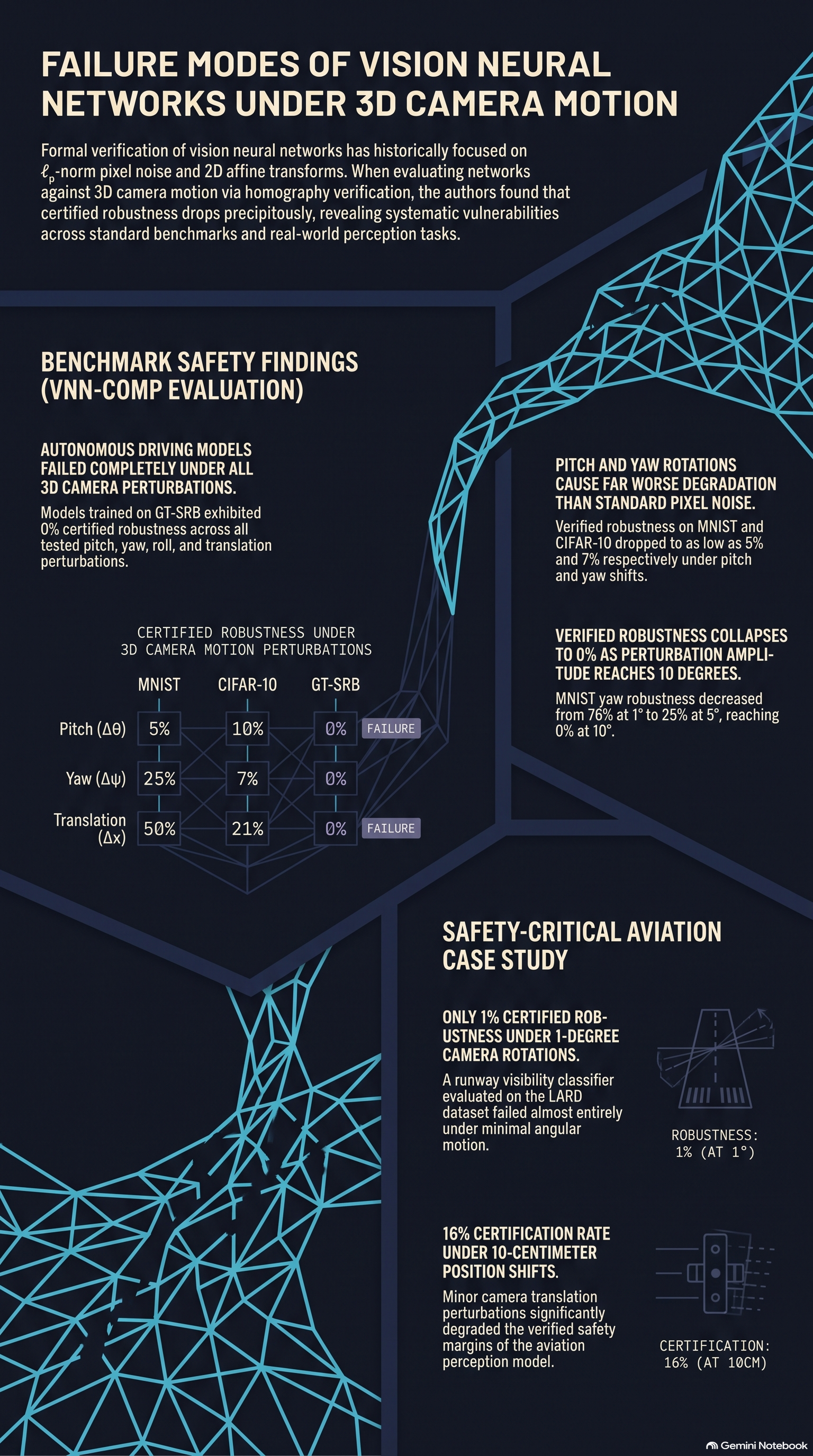
The evaluation demonstrated that networks certified against standard adversarial perturbations remain highly vulnerable to 3D camera pose shifts.

Perturbation	Parameter Interval $B$	MNIST Robustness (%)	CIFAR-10 Robustness (%)	GT-SRB Robustness (%)	Generation Time (s)	Verification Time (s)	Total Timeouts
Roll ($\Delta\phi$)	$[0, 5]^\circ$	61	69	0	—	—	—
Pitch ($\Delta\theta$)	$[0, 5]^\circ$	5	10	0	—	—	—
Yaw ($\Delta\psi$)	$[0, 5]^\circ$	25	7	0	—	—	—
Translation $\Delta x$	$[0, 1]\text{ m}$	50	21	0	—	—	—
Translation $\Delta y$	$[0, 1]\text{ m}$	73	83	0	—	—	—
Translation $\Delta z$	$[0, 1]\text{ m}$	53	24	0	—	—	—
Dataset Totals / Overhead	—	—	—	—	42.0	8.23	0
MNIST	—	—	—	—	1858.6	41.33	2
CIFAR-10	—	—	—	—	292.6	5323.8	178
GT-SRB	—	—	—	—	—	—	—

The empirical results reveal crucial insights into geometric robustness:

1. Matrix Properties Drive Robustness Disparities: Models exhibit markedly higher robustness to roll ($\Delta\phi$) and lateral translation ($\Delta y$). Under the authors’ coordinate system choices, the inverse homography matrices $H^{-1}(\Delta\phi)$ and $H^{-1}(\Delta y)$ contain a bottom row of $[0, 0, 1]$. Consequently, depth normalization becomes trivial ($h_3(\kappa) = 1$), causing the transformations to simplify into exact 2D affine rotation and shear. Standard data augmentation techniques cover these affine variations relatively well.
2. Systematic Failure Under Perspective Shifts: Pitch ($\Delta\theta$), yaw ($\Delta\psi$), and translations $\Delta x, \Delta z$ force $h_3(\kappa)$ to depend non-linearly on spatial coordinates. This dependency induces spatial perspective scaling that standard $\ell_p$-norm adversarial training (e.g., PGD) cannot defend against.
3. GT-SRB Collapse and MILP Bottlenecks: The GT-SRB traffic sign classifier achieved 0% certified robustness across every tested 3D motion parameter. Furthermore, GT-SRB verification produced 178 timeouts (out of 600 evaluated properties). As Durand et al. explain, these timeouts reflect severe MILP solver bottlenecking within VENUS caused by larger input dimensions, deeper model architectures, and unconstrained ReLU node states.

---

6. Safety-Critical Case Study: Autonomous Runway Visibility Classification

To demonstrate the real-world implications of these vulnerabilities, Durand et al. conducted a case study on an aerospace vision model. The target system was a binary neural network classifier trained on the Landing Approach Runway Detection (LARD) dataset. This model predicts runway visibility during approach to inform pilot go-around decisions in accordance with aviation safety guidelines.

When subjected to formal homography verification, the runway classifier demonstrated extreme fragility to minor camera displacements:

• Only 16% of test images maintained certified robustness under a small 10 cm translation.
• Only 1% of test images remained certified robust under a 1° camera rotation.

Perception models deployed in safety-critical domains like aerospace require explicit formal certification against 3D camera motion, as standard training leaves them vulnerable to minor physical camera displacements.

---

7. Sensitivity, Limitations, and Practical Scope

The verification framework proposed by Durand et al. operates within specific mathematical boundary conditions:

1. Planar Scene Assumption: The formulation explicitly models plane-to-plane mappings. It is designed for predominantly planar scene features—such as ground planes in Inverse Perspective Mapping, airport runways, traffic signs, and planar robotic workspaces—where parallax effects and object occlusions are minimal.
2. Sensitivity to Transform Amplitude: Bounding non-linear pixel trajectories becomes challenging as angular perturbations grow. On the MNIST dataset, certified robustness under yaw perturbations dropped from 76% at 1° to 25% at 5°, reaching 0% at 10° or greater.
3. Impact of Padding Techniques: Transformed pixel coordinates frequently fall outside original image boundaries, requiring padding imputation. Durand et al. evaluated five distinct padding methods (Black, Gray, Replicate, Reflect, Wrap) on CIFAR-10 under yaw perturbations:
   • At $2.5^\circ$ yaw, perceptually plausible padding techniques preserved higher certified robustness (Reflect: 42%, Replicate: 42%) than stark borders (Black: 34%, Gray: 33%, Wrap: 35%).
   • At $5.0^\circ$ yaw, robustness collapsed across all padding mechanisms (Black: 7%, Gray: 7%, Replicate: 8%, Reflect: 9%, Wrap: 7%). This demonstrates that while plausible padding mitigates border artifacts at minor angles, it cannot prevent robustness failure as projective distortions scale.

---

8. Conclusion & Strategic Insights for AI Safety Red-Teamers

The findings by Durand et al. provide essential lessons for researchers auditing the safety and reliability of vision models:

• $\ell_p$-Norm Metrics Leave Safety Gaps: Standard pixel-noise robustness guarantees do not translate to physical safety when sensors undergo 3D spatial rotation or translation.
• Homographies Provide Tractable 3D Bounds: Homographic formulations offer a closed-form, mathematically sound mechanism to verify physical camera motion on planar scene elements without requiring full 3D mesh rendering or neural surrogate models.
• Targeted Geometric Defense is Mandatory: Passing real-world safety certification requires incorporating specialized robust training protocols or 3D projective data augmentations targeted at 6-DOF camera pose variations.

Code and implementation details for this homography verification framework are publicly available at https://github.com/jeangud/homography-verification.

Read the full paper on arXiv · PDF